S E6000C Mini-OTDR User’s Guide S1
Notices Warranty Edition/Print Date Copyright © 2000, 2001 Agilent Technologies Deutschland GmbH. All rights reserved. The material contained in this document is subject to change without notice. Agilent Technologies makes no warranty of any kind with regard to this material, including, but not limited to, the implied warranties of merchantability and fitness for a particular purpose.
Safety Summary Safety Summary The following general safety precautions must be observed during all phases of operation of this instrument. Failure to comply with these precautions or with specific warnings elsewhere in this manual violates safety standards of design, manufacture, and intended use of the instrument. Agilent Technologies assumes no liability for the customer’s failure to comply with these requirements.
Safety Summary FUSES Only fuses with the required rated current, voltage, and specified type (normal blow, time delay, etc.) should be used. Do not use repaired fuses or short-circuited fuse holders. To do so could cause a shock or fire hazard. DO NOT OPERATE IN AN EXPLOSIVE ATMOSPHERE Do not operate the instrument in the presence of flammable gases or fumes. DO NOT REMOVE THE INSTRUMENT COVER Operating personnel must not remove instrument covers.
Safety Summary Symbols Caution, refer to accompanying documents Hazardous laser radiation Electromagnetic interference (EMI) E6000C Mini-OTDR User’s Guide, E0302 5
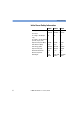
Safety Summary Initial Laser Safety Information Laser Type Laser Class According to IEC 825 (Europe) According to 21 CFR 1040.10 (Canada, Japan, USA) Output Power (Pulse Max) Pulse Duration (Max) Pulse Energy (Max) Output Power (CW) Beam Waist Diameter Numerical Aperture Wavelength 6 E6001A E6003A E6003B FP-Laser InGaAsP FP-Laser InGaAsP FP-Laser InGaAsP 3A 3A 3A 1 1 1 50 mW 10 µs 500 nWs 500 µW 9 µm 0.1 1310 ±25nm 50 mW 10 µs 500 nWs 500 µW 9 µm 0.
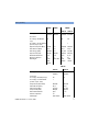
Safety Summary E6004A E6007A E6008B 1310 nm Laser Type Laser Class According to IEC 825 (Europe) According to 21 CFR 1040.10 (Canada, Japan, USA) Output Power (Pulse Max) Pulse Duration (Max) Pulse Energy (Max) Output Power (CW) Beam Waist Diameter Numerical Aperture Wavelength 1550 nm FP-Laser InGaAsP MQW-Laser FP-Laser FP-Laser AlGaInP InGaAsP InGaAsP 3A 2 3A 3A 1 2 1 1 50 mW 10 µs 500 nWs 500 µW 9 µm 0.1 1310/ 1550 ±25nm n/a n/a n/a 500 µW 9 µm 0.1 635 ±10nm 120 mW 20 µs 2.
Safety Summary E6005A / E6009A Laser Type Laser Class According to IEC 825 (Europe) According to 21 CFR 1040.10 (Canada, Japan, USA) Output Power (Pulse Max) typ ≤ 30 ns Output Power (Pulse Max) typ > 30 ns Pulse Duration (Max) Pulse Energy (Max) Output Power (CW) Beam Waist Diameter Numerical Aperture Wavelength 1300 nm 850 nm FP-Laser InGaAsP MOCVD GaAlAs 3A 1 3A 1 20 mW 10 mW 10 µs 200 nWs 50 µW 50 µm 0.2 1300 ±25nm 40 mW 20 mW 100 ns 4 nWs 20 µW 62.5 µm 0.
Safety Summary Non-USA The following symbol is fixed to the panel of the MiniOTDR modules, next to the laser output: A sheet of laser safety warnings is included with the laser module. You must stick the labels in the local language onto the outside of the instrument, in a position where they are clearly visible to anyone using the instrument.
Safety Summary Submodule E6007A The laser safety labels for the USA, according to 21 CFR 1040.10 Class II, are already attached to the module. A sheet of laser safety warnings is included with the laser module. You must stick the labels in the local language onto the outside of the instrument, in a position where they are clearly visible to anyone using the instrument. All modules also have a CE class A label.
About This Manual About This Manual The Structure of this Manual This manual is divided into 4 parts: • “Getting Started” on page 31 tells you how to set up your Mini-OTDR. • “Additional Features” on page 67 shows you what you can do with your Mini-OTDR. • The Sample Sessions (starting “Sample Sessions: Measuring a Trace” on page 81) give you a step-bystep guide to making typical measurements and using other Mini-OTDR features.
Service and Support • E4310-91016 Agilent Technologies OTDRs Programming Guide • E6000-91017 Agilent OTDRs Pocket Guide • 5963-3538F Cleaning Procedures for Lightwave Test and Measurement Equipment: Pocket Guide 6HUYLFH DQG 6XSSRUW Any adjustment, maintenance, or repair of this product must be performed by qualified personnel. Contact your customer engineer through your local Agilent Technologies Service Center. You can find a list of local service representatives on the Web at: http://www.agilent.
Service and Support New Zealand 0800 738 378 64 4 495 8950 (FAX) Asia-Pacific (852) 3197 7777 (852) 2506 9284 (FAX) E6000C Mini-OTDR User’s Guide, E0302 13
Service and Support 14 E6000C Mini-OTDR User’s Guide, E0302
E6000C Mini-OTDR User’s Guide Safety Summary Symbols Initial Laser Safety Information Safety Labels About This Manual Service and Support 1 Getting Started 1 3 5 6 8 11 12 31 Features of the Mini-OTDR The Front panel The hardkeys External Markings The Mini-OTDR module Removing a Module Inserting a Module Adding a Connector Interface Switching on the Mini-OTDR The Applications Screen OTDR Mode Taking a Measurement The parameter windows The Cursor and Select keys The popup panel Zooming The Settings s
2 Additional Features 67 How the OTDR Works Events What You Can Measure with the OTDR External connections 67 68 69 70 71 Switches Inserting and Removing a Floppy Disk, Flash Disk, or SRAM Card 72 Adding a Shoulder Strap 73 Inserting and Removing a Submodule 74 Battery Handling Inserting and Removing a Battery Charging the Batteries Battery Storage Battery safety Connecting an AC/DC Adapter The Mini-Keyboard 3 Sample Sessions: Measuring a Trace How to Connect the Fiber How to Change the Refractive I
How to Set the Horizontal Offset How to Hide Events before the Offset How to Clear the Horizontal Offset How to Set the Fiber End How to Print the Measurement How to make a screen dump How to Save the Measurement 4 Sample Sessions: Analyzing an Existing Trace How to Add a Landmark or Event Comment How to Add a Landmark How to Add an Event Comment How to Add a Reflective Event 96 98 98 98 100 103 104 107 108 108 110 111 How to Set the Level-Markers for Measuring Reflectance 112 How to Set the Level-mar
How to Set the Default Trace Information How to Set the Information for the Current Trace How to Update the Firmware How to Update the Languages 136 138 139 140 141 142 144 145 145 6 Sample Sessions: Other Mini-OTDR Modes 149 How to Connect to a PC using the RS232 How to Set the Instrument Setup How to Set up the Printer Configuration How to Add a Logo How to Update the Firmware and Languages How to Recall Settings in EasyMode How to Save a Template How to Read from a Presaved Template How to set u
How to Use the Visual Fault Finder submodule A Installation and Maintenance Safety Considerations Initial Inspection Internal Back-Up Battery AC Line Power Supply Requirements Line Power Cable DC Power Supply Requirements Operating and Storage Environment Temperature and Humidity Altitude Installation Category Parallel Interface Serial Interfaces Programming user tasks on a PC Claims and Repackaging Return Shipments to Agilent Technologies Installing New Firmware B Accessories 171 175 175 176 176 177
Distance accuracy 194 Distance offset error 195 Distance sampling error 197 Distance scale error 198 Dynamic range (RMS) 199 Event deadzone 200 Group index (of a fiber) 200 Loss accuracy, backscatter measurements (1 dB steps) 201 Loss accuracy, reflectance measurements Noise level (98%) Noise level (RMS) Output power (CW) Output power stability (CW) Reflectance accuracy Sample spacing Signal-to-noise ratio (SNR) Definition of Terms - Power Meter Submodule Definition of Terms - Visual Fault Finder Submodule
Specifications: Optical Performance Characteristics Agilent E6006A Power Meter Submodule Characteristics Specifications Supplementary Performance Characteristics General Specifications: Agilent E6007A Visual Fault Finder Submodule Characteristics Supplementary Performance Characteristics General Specifications: Declaration of Conformity D Single-Mode/Multimode Module Performance Tests 211 213 214 214 215 215 216 217 217 217 217 218 219 General 219 Equipment Required 219 Test Record 220 Test Failure 2
E Cleaning Information 271 Cleaning Instructions for this Instrument 271 Safety Precautions 273 Why is it important to clean optical devices ? 274 What do I need for proper cleaning? 274 Standard Cleaning Equipment 275 Additional Cleaning Equipment 279 Preserving Connectors 281 Making Connections 281 Dust Caps and Shutter Caps 282 Immersion Oil and Other Index Matching Compounds 283 Cleaning Instrument Housings Which Cleaning Procedure should I use ? Light dirt Heavy dirt How to clean connectors Preferr
interface 290 How to clean instruments with an optical glass plate 291 How to clean instruments with a physical contact interface 291 Preferred Procedure Procedure for Stubborn Dirt 292 292 How to clean instruments with a recessed lens interface 293 Preferred Procedure Procedure for Stubborn Dirt 293 293 How to clean optical devices sensitive to mechanical 294 stress Preferred Procedure Procedure for Stubborn Dirt Alternative Procedure 294 294 295 How to clean metal filters or attenuator gratings 295
Agilent Technologies Manufacturing Process G Overview 305 H Appendix: VENDOR.
Figure 1 Figure 2 Figure 3 Figure 4 Figure 5 Figure 6 Figure 7 Figure 8 Figure 9 Figure 10 Figure 11 Figure 12 Figure 13 Figure 14 Figure 15 Figure 16 Figure 17 Figure 18 Figure 19 Figure 20 Figure 21 Figure 22 Figure 23 Figure 24 Figure 25 Figure 26 Figure 27 Figure 28 Figure 29 Figure 30 Figure 31 Figure 32 Figure 33 Figure 34 Figure 35 Figure 36 Figure 37 Figure 38 Figure 39 Figure 40 The Front Panel . . . . . . . . . . Mini-OTDR hardkeys . . . . . . . . . The Mini-OTDR module . . . . . . . .
Figure 41 Figure 42 Figure 43 Figure 44 Figure 45 Figure 46 Figure 47 Figure 48 Figure 49 Figure 50 Figure 51 Figure 52 Figure 53 Figure 54 Figure 55 Figure 56 Figure 57 Figure 58 Figure 59 Figure 60 Figure 61 Figure 62 Figure 63 Figure 64 Figure 65 Figure 66 Figure 67 Figure 68 Figure 69 Figure 70 Figure 71 Figure 72 Figure 73 Figure 74 Figure 75 Figure 76 Figure 77 Figure 78 Figure 79 Figure 80 26 Measuring Insertion Loss: setting the level-markers . . . Declaring an End at the edge of the backscatter .
Figure 81 Figure 82 Figure 83 Figure 84 Figure 85 Figure 86 Figure 87 Figure 88 Figure 89 Figure 90 Figure 91 Figure 92 Figure 93 Figure 94 Attenuation Deadzone Test: Position Marker A . . . . Attenuation Deadzone Test: Marker B at End of Reflection . Attenuation Deadzone Test: Marker A at Start of Reflection. Distance Accuracy Test Setup . . . . . . . . Distance Accuracy Test: Position Markers . . . . . Distance Accuracy Test: Around Marker View . . . .
E6000C Mini-OTDR User’s Guide, E0302
E6012A, E6013A) Table 1 Table 2 Table 3 225 Table 4 Table 5 Table 6 Mini-OTDR: External Markings . . . . . . . . . 34 Dynamic Range Test settings: single-mode (E6001A to E6004A) 225 Dynamic Range Test settings: single-mode (E6003B, E6008B, Dynamic Range Test settings: multimode . . Power Meter: Test Equipment Required . . Visual Fault Finder: Test Equipment Required . E6000C Mini-OTDR User’s Guide, E0302 . . . . . . . . . .226 .258 .
E6000C Mini-OTDR User’s Guide, E0302
1 1 Getting Started Getting Started introduces the features of the Agilent Technologies E6000C Mini-OTDR (Optical Time Domain Reflectometer). Here you will find a quick description of the instrument, an explanation of how to insert a module and Connector Interface, and a description of the main Mini-OTDR screens. This manual is also valid for the Agilent E6000B MiniOTDR. Some new features, not available with the E6000B are also described.
1 Getting Started Features of the Mini-OTDR Battery Charging Power On Figure 1 • The red battery charging light is lit when the battery is charging. • The green power on light is lit when the power is on. The Front Panel The hardkeys There are four keys on the front of the Mini-OTDR. Run/Stop 32 • The blue RUN/STOP key starts or stops a trace acquisition. Cursor • The CURSOR keys enable you to navigate around the menu system, or to move markers and so on.
Features of the Mini-OTDR 1 Getting Started Help • The HELP key, marked ?, gives you information about the currently highlighted object. If no object is highlighted, you see more general help information. The RUN/STOP and HELP keys do not change their meaning wherever you are in the menu system. The CURSOR keys and the SELECT key can be used for more specific purposes. The current interpretation of these keys is shown in the diagram at the right of the screen .
1 Getting Started External Markings External Markings You see the following external markings on the MiniOTDR: Table 1 Mini-OTDR: External Markings Marking Explanation More Info Battery charging light “The Front panel” on page 31 Power on light Power on switch DC Input Connector “Switches” on page 71 Contrast Switch Backlight ON/OFF Serial Interface Parallel Interface “Serial Interfaces” on page 181 “Parallel Interface” on page 180 DC label CE label 34 E6000C Mini-OTDR User’s Guide, E0302
The Mini-OTDR module 1 Getting Started The Mini-OTDR module Figure 3 shows a Mini-OTDR with a module inserted in the back. Figure 3 The Mini-OTDR module Module catches • You keep the module in place with the module catches. When the module is in place, the catches should be perpendicular to the screen. Connect fiber • You connect fibers to the Optical Output Connector. For more details, see “Adding a Connector Interface” on page 38. Submodule • You add submodules to the submodule slot.
1 Getting Started The Mini-OTDR module Removing a Module N O TE Figure 4 You should switch off your Mini-OTDR before inserting or removing a module or submodule. Removing a module Module slot The slot in the back of the Mini-OTDR is used for the various Mini-OTDR measurement modules. When you are inserting or removing a module, open the connector covers at the top of the module.
The Mini-OTDR module 1 Getting Started Remove module 3 Pull the module out of the module slot. When the module has been fully removed, turn the catches 90 degrees so that they are perpendicular to the screen. Inserting a Module NOTE You should switch off your Mini-OTDR before inserting or removing a module or submodule. Module slot The slot in the back of the Mini-OTDR is used for the various Mini-OTDR measurement modules.
1 Getting Started The Mini-OTDR module Adding a Connector Interface Figure 5 Adding a Connector Interface Before you add the connector interface, you must have inserted a module to your Mini-OTDR. On the left of the module when viewed from behind, you see an Optical Output Connector (see Figure 5). N O TE Before you attach a connector and fiber, you should clean them both. See “How to clean connectors” on page 284 and “How to clean bare fiber adapters” on page 288.
Switching on the Mini-OTDR 1 Getting Started Switching on the Mini-OTDR Self test When you switch on the Mini-OTDR it goes through self test. If the Mini-OTDR indicates a problem with the module, switch off the instrument, make sure the module is properly inserted and snapped into the Mini-OTDR, and try switching the instrument on again. Check power supply If you have no reaction, check that the machine is connected to a power source (AC/DC adapter or battery). See “Battery Handling” on page 75.
1 Getting Started The Applications Screen Figure 6 Application Modes The Applications Screen There are 9 different applications for different tasks and user groups: • OTDR Mode contains all the features for making, viewing, and analyzing traces. OTDR mode gives you the full functionality of a “classical” OTDR. See “OTDR Mode” on page 41. • Fiber Break Locator is a simplified trace setting that enables you to locate fiber breaks quickly.
OTDR Mode 1 Getting Started • Easy OTDR enables you to view a trace, and to perform simple operations like Print and apply presaved settings. See “EasyMode” on page 62. • Multi Fiber Test allows you to define up to 4 measurements, and apply all measurements to multiple fibers (for example, all fibers in a cable).
1 Getting Started OTDR Mode Figure 7 Blank Trace Screen Taking a Measurement N O TE Before you take a measurement you should attach a fiber to the Connector Interface. See “Adding a Connector Interface” on page 38. To produce a trace, press the RUN/STOP hardkey. Run/Stop light Stop measurement. 42 The light behind the RUN/STOP hardkey goes on.
OTDR Mode 1 Getting Started . Figure 8 The Trace Screen Trace • When you have taken a measurement, the graph of the reflected power is displayed as a function of distance. This graph is called the trace. Event Bar • Below the trace, the event bar shows you the position of the detected events: non-reflective events such as splices, reflective events such as connectors, as well as any defined landmarks. You can add and remove the event bar by selecting [View] from the popup panel.
1 Getting Started OTDR Mode Trace Overview • No matter when you zoom to a point of interest on the trace, you do not lose orientation, as there is an overview display in the full-trace window. You always know where you are. The full-trace window is shown in the bottom left-hand corner of the display. In the title bar you can see the name of the measurement file (UNNAMED if you have not already saved the measurement).
OTDR Mode Relative to both markers 1 Getting Started The following parameters are measured between marker A and marker B. The recorded values change when you move either marker. • A-B: the distance between the markers • One of the following (selectable in the [ANALYSIS] menu): – 2pt.L: 2-point loss between the markers. This is the difference in power level between the marker points – 2pt.Attn.: 2-point attenuation. This is the 2-point loss per length unit. – LSA-Attn.: LSA Attenuation.
1 Getting Started OTDR Mode • PWidth: The pulsewidth in seconds (ns or µs), selectable from the [SETTINGS] menu. The available pulse widths are module-dependent. • Optimize: The Optimizing mode. This is the range for measurements, and is selectable from the [SETTINGS] menu. Possible Optimizing modes are – Resolution: for short fibers, – Dynamic: for long fibers, and – Standard: for a compromise between Resolution and Dynamic. If you have specified Automatic measurements, you see Auto Res., Auto Dyn.
OTDR Mode 1 Getting Started Cursor Down • The DOWN key zooms in around the current marker, which stays in the center of the grid. If both markers are highlighted, zooming is performed around the midpoint of the markers. Pressing the DOWN key for a second time restores the full trace. The Cursor key diagram to the right of the trace shows the current mode. If you see a horizontal magnifying glass, you are viewing the whole trace.
1 Getting Started The popup panel The popup panel If you press the SELECT key in OTDR mode. you normally see a popup panel, offering fast access to various menus and important functions. Figure 10 The popup panel The following functions are available in OTDR mode: • [CANCEL] - exit the popup panel and return to normal OTDR mode. • [FILE] menu - File utilities, including loading and storage of data and printing a trace. • [CONFIG] menu - configure the Mini-OTDR.
The popup panel 1 Getting Started • [ANALYSIS] menu - analyze the trace. Use the cursor keys to move to the function you require, and press SELECT again to select it. NOTE If you do not select any option, the popup panel disappears after approximately 10 seconds. When you select [FILE], [CONFIG], [VIEW], [EVENTS], or [ANALYSIS], you see a list of menu options. Use the UP and DOWN cursors to move to the option you want, and press SELECT or RIGHT.
1 Getting Started The Settings screen The Settings screen Select SETTINGS from the popup panel. You see one of the two pages of the Settings screen: Measurement Settings or Pass/Fail Parameters. Change Settings screen Figure 11 Change parameters You switch between the Settings pages by selecting one of the arrows at the bottom left of the Settings screen (Figure 11). Settings page navigation arrows To change a parameter in the settings screen, move to the appropriate box and press SELECT.
The Settings screen 1 Getting Started NOTE Changes made to the settings screen only affect subsequent measurement acquisitions. However, you can apply the changes that you have made to a trace that is currently running by pressing RUN/STOP again. The Measurement Settings screen The Measurement Settings page contains a list of parameters that you can set (Figure 12).
1 Getting Started The Settings screen Wavelength • Wavelength: laser wavelength. This is only meaningful if you have a dual-wavelength OTDR module. The available wavelengths depend on how your module has been configured. Measurement Mode • Meas. Mode: The Measurement Mode: Realtime to update the settings while making a measurement, Averaging to reduce noise level (normal OTDR measurement mode), or Continue to continue averaging a measurement that you have stopped.
The Settings screen 1 Getting Started Averaging Time • Avg. Time: Averaging time of a measurement. The measurement is stopped automatically when this time has elapsed. Larger Averaging Times increase the dynamic range by reducing the noise floor of the OTDR. The specified dynamic range is reached after 3 minutes. NOTE This parameter can also be configured to be Number of Averages: a specified number of measurement acquisitions. Number of Averages is a power of 2.
1 Getting Started The Settings screen N O TE The way in which the Reflectance and Front Connector Thresholds are calculated depends on how you have configured the Reflectance Parameter in the Instrument Config OTDR Settings screen (see “How to Set the OTDR Settings” on page 134). A Reflection Height Threshold value of 0.0 dB, or a Front Connector Threshold value of -.- dB means that the Threshold is not checked. Non-Reflectance Threshold End Threshold • NonRefl Thres: the Non-Reflectance Threshold.
The Settings screen 1 Getting Started Figure 13 The Pass/Fail Parameters Settings page You can change the following parameters from this page: Non-Reflectance Limit • NRefl. Limit: Non-Reflectance Limit. All Events with an Insertion Loss greater than this limit are reported in the Pass/Fail test Table. Gainers are never entered in the Pass/Fail test table. This is because it is not possible to accurately measure the true Insertion loss of a gainer without taking a twoway Averaging Measurement.
1 Getting Started The Settings screen active, you see a value of -.- dB in the Refl. Limit edit field. Connector Loss Limit • Conn. Loss Limit: Insertion Loss for the Connector. A Pass/Fail test checks whether any Reflective Events have an Insertion Loss greater than this limit. For all Events which exceed the limit, you see an entry in the Pass/Fail Test table. So, if the Connector Loss limit is 0.8dB, all Events with an Insertion Loss greater than 0.8dB are entered in the Pass/Fail Test table.
The Settings screen 1 Getting Started Total Link Loss • Total Link Loss: Loss over whole fiber. This is calculated as the loss between the Horizontal Offset (see “How to Set the Horizontal Offset” on page 96) and the Fiber End. An End Event must be present before this test can be performed. See “How to Set the Fiber End” on page 98. If the Loss between the Horizontal Offset and the Fiber End is greater than this limit, this is reported in the Pass/Fail test table.
1 Getting Started The Settings screen not appear in the Event Table, they are reported in the Pass/Fail test table. If you select New Events, you should also set at least one other parameter in the Pass/Fail Param. window. This feature is best used with a locked Event Table. See “How to Lock the Event Table” on page 91. The check for New Events uses the current Scan Trace thresholds. Link Length • Link Length: Distance to Fiber End.
The File Utilities screen 1 Getting Started limit is not active, you see a value of -.--- km in the Link Tolerance edit field. If no Length Tolerance is set, the distance between the Horizontal Offset and the Fiber End must be exactly the same as the Link Length. If no Link Length has been set, the value of the Length Tolerance is irrelevant. Event Masking • Event Masking: Specify events to be masked. See “How to Mask Events” on page 92.
1 Getting Started The File Utilities screen Figure 14 Search for files The File Utilities screen You can use the UP and DOWN cursors to look at files on the current device (by default, this is the Mini-OTDR’s internal directory structure). At the bottom of the screen, you see information about the currently highlighted file. Press SELECT to select the highlighted file or directory. When a file is selected, you see a tick next to it. You may select as many files as you like.
The File Utilities screen 1 Getting Started Copy: Copy the currently selected file(s). When you select this option, you may choose a new directory or a different device. If no file is selected, this option is grayed. Print: Print the currently selected file(s). You must have a printer connected to the Mini-OTDR. For more information, see “How to Print the Measurement” on page 100. If no file is selected, this option is grayed. NOTE You may only print traces. Traces usually have the extension .SOR, .
1 Getting Started EasyMode If you try to format the internal device, your configuration is lost and your Mini-OTDR must be reconfigured. Delete directory RmDir: Delete a directory. After you have selected RmDir move to the directory you want to delete, changing device if necessary. Then cursor RIGHT to Delete and press SELECT. N O TE You cannot delete a directory if there are any files in that directory. Create directory MkDir: Create a new directory.
EasyMode 1 Getting Started Figure 15 EasyMode popup panel EasyMode popup panel The following functions are available on the EasyMode popup panel: • [CANCEL] - exit the popup panel. • [SAVE] - save the current file. [SAVE] is equivalent to [FILE] in OTDR mode. See “How to Save the Measurement” on page 104 • [PRINT]- print the current trace. [PRINT] is equivalent to [FILE] in OTDR mode. See “How to Print the Measurement” on page 100.
1 Getting Started Getting Help Settings file A settings file (“.SET”) just contains values from the Settings menu. See the note on page 50. • [OFFSET] - change the offset. Use the cursors to move the vertical position of the trace on the screen. [OFFSET] is equivalent to [VIEW] in OTDR Mode. • [CLOSE] - return to Applications Screen, as in the OTDR Mode popup panel option. • [EVENTS] - show or hide the Event Table. Equivalent to [VIEW] in OTDR mode.
Getting Help 1 Getting Started Figure 16 The Mini-OTDR’s Help Display To leave the online documentation and resume your task, press the HELP key again. Alternatively, cursor right to Done and press SELECT.
1 Getting Started 66 Getting Help E6000C Mini-OTDR User’s Guide, E0302
2 2 Additional Features Additional Features introduces additional features of the Agilent Technologies E6000C Mini-OTDR (Optical Time Domain Reflectometer). Here you will find descriptions of how an OTDR works, and how you can add external features to your Mini-OTDR. How the OTDR Works The OTDR repeatedly outputs an optical pulse into the connected fiber and measures the reflections from this pulse.
2 Additional Features Events Events Events are changes in the fiber causing the trace to deviate from a straight line. Events can be Reflective or Non-Reflective. Reflective Events Reflective Events occur when some of the pulse energy is reflected, for example at a connector. Reflective Events produce a spike in the trace (you see a steep rise and fall in the graph: see the first diagram below).
Events 2 Additional Features What You Can Measure with the OTDR The OTDR displays the relative power of the returned signal against distance.
2 Additional Features External connections greater than the End Threshold. See “How to Set the Fiber End” on page 98 for more details. As a result, the event parameters’ loss, reflectance, and distance are calculated and listed. External connections Figure 17 shows the external connections to the MiniOTDR. There are 3 flaps on top of the Mini-OTDR: Figure 17 Flaps at top of Mini-OTDR Mini-OTDR external connections – Under the left flap you see switches. See “Switches” below.
External connections 2 Additional Features Removing a Floppy Disk, Flash Disk, or SRAM Card” on page 72. – Under the right flap you see interfaces to connect with Centronics and RS232. Shoulder strap • You can attach a shoulder strap to points on either side of the Mini-OTDR. See “Adding a Shoulder Strap” on page 73. Battery • You insert the battery behind the flap in the bottom right corner of the Mini-OTDR. See “Inserting and Removing a Battery” on page 75.
2 Additional Features External connections Brightness • You change the brightness of the picture with the backlight button. Contrast • You change the contrast of the picture with the contrast switch. Input connector • You use the DC input connector when you want to attach an AC/DC connector. See “Connecting an AC/DC Adapter” on page 78 for more details. Power on • You turn the Mini-OTDR on and off with the power on switch.
External connections 2 Additional Features NOTE Please make sure that the disk that any floppy disks that you insert are pre-formatted. The Mini-OTDR will not format disks, and does not recognize unformatted disks. Adding a Shoulder Strap Figure 20 Adding hinges for the shoulder strap You can attach a shoulder strap to the connection points on the left and right sides of the Mini-OTDR.
2 Additional Features External connections Inserting and Removing a Submodule N O TE Figure 21 You should switch off your Mini-OTDR before inserting or removing a module or submodule. Inserting a submodule Module 1 Insert a module The submodules E6006A and E6007A go in the submodule slot at the top of main Mini-OTDR modules. Follow the steps in “Inserting a Module” on page 37.
Battery Handling 2 Additional Features The submodule slips easily in and out of its slot (Figure 21). When the submodule is in place, you can now connect an Optical Output Connector and a fiber, and lock the module. Battery Handling Inserting and Removing a Battery The battery should be inserted in the slot at the foot of the Mini-OTDR (see Figure 22.) NOTE Make sure that you insert the battery in the correct direction, and that you close the battery cap correctly.
2 Additional Features Battery Handling . Figure 22 Removing a Battery Once you have inserted or removed the battery, replace the cap C A UT IO N Do not insert the battery while operating the instrument. Charging the Batteries The Mini-OTDR has a built-in charger. It is able to charge the battery operating or non-operating. Fast-charge is typically performed non-operating in 2 hours.
Battery Handling 2 Additional Features Best performance • For the best battery performance and accuracy of the fuel gauge (showing percentage use of the battery), completely discharge the battery, then make a complete fast charge cycle (non-operating), and completely discharge the battery again. NOTE You must ensure that the charging cycle is not interrupted by a battery discharge, and that the discharge cycle is not interrupted by battery charging.
2 Additional Features Battery Handling • The battery can explode, leak or catch fire if heated or exposed to fire or high temperatures. • Do not short circuit the battery by directly connecting the metal terminals (+,-). Be certain that no metal objects such as coins, paper clips and so on touch the terminals. • Do not drop the battery or subject it to mechanical shock. N O TE The battery is a consumable part and is not subject the E6000C warranty.
The Mini-Keyboard Input connector 2 Additional Features You see an input connector next to the On/Off button. Attach the lead from the charger to this connector (Figure 23). The Mini-Keyboard If you order the Agilent E6081A, you receive a PS2 keyboard, that you can attach at the back of your MiniOTDR, to the right-hand side (see Figure 24). You can use the keyboard in place of the screen keyboard to enter text (see, for instance, “How to change a text setting” on page 132).
2 Additional Features Figure 24 The Mini-Keyboard Attaching a keyboard You can use a mini-DIN connector to attach any standard PS2 keyboard, such as the Agilent E6081A, to the keyboard connector.
3 3 Sample Sessions: Measuring a Trace Measuring a Trace contains a number of sample sessions of step-by step guides showing how to use common features of the Mini-OTDR. Equipment used In these sample sessions we use: • A Mini-OTDR Agilent Technologies E6000C with an optical module Agilent E6003A (1310/1550 nm, singlemode). • A length of fiber of about 40 km, terminated at one end with a Diamond HMS-10/Agilent connector and unterminated at the other end. The fiber has a refractive index of 1.
3 Sample Sessions: Measuring a Trace How to Connect the Fiber • Print and Save the Measurement. How to Connect the Fiber Connecting the fiber to the Mini-OTDR is very easy. You do not need any tools. 1 Clean the connectors. See “How to clean connectors” on page 284. 2 Attach the required optical connector interface to the optical output. See “Adding a Connector Interface” on page 38. 3 Connect the fiber to this interface. 4 Turn on the Instrument.
How to Change the Refractive Index Setting Measurement Settings 3 Sample Sessions: Measuring a Trace 2 Select [SETTINGS] from the popup panel. You see a menu headed Measurement Settings. 3 If you are not already viewing the Meas. Parameter page, cursor to either of the arrows at the bottom left of the screen. Press SELECT to bring up the next page. Select Refractive Index 4 Use the Cursor keys to move to the box, and press SELECT.
3 Sample Sessions: Measuring a Trace How to Make an Automatic Measurement 6 Move to OK in the Measurement Settings menu and press the SELECT key. N O TE Parameters changed in the [SETTINGS] page only affect subsequent traces. The current trace is unaltered. If you alter the settings while a measurement is running, press RUN/STOP again to start a new trace with the parameters that you have just set. N O TE You can alter the Refractive Index Setting for just the current trace by selecting
How to Make an Automatic Measurement 3 Sample Sessions: Measuring a Trace Automatic Settings 3 Cursor up to and press SELECT. Automatic settings are now enabled. You see the text Auto in the Range and PulseWidth boxes, and the Mini-OTDR selects suitable settings for your fiber. 4 Exit the SETTINGS menu by selecting OK. Automatic Scanning 5 Select [VIEW] from the popup panel. You see a list of menu options. 6 If there is a tick next to , Automatic Scanning is already enabled.
3 Sample Sessions: Measuring a Trace How to Run a Manual Measurement How to Run a Manual Measurement When you already know about the fiber under test, you can set the parameters exactly. This section describes how to setup and run a measurement manually. How to Change the Measurement Span 1 Select [SETTINGS] from the OTDR Mode popup panel. 2 If you are not already viewing the Meas. Parameter page (Figure 12), cursor to either of the arrows at the bottom left of the screen.
How to Run a Manual Measurement 3 Sample Sessions: Measuring a Trace bottom left of the screen. Press SELECT to bring up the next page. Optimize Mode 3 Move to and press SELECT. You see three options: , and . 4 If you want to increase the dynamic range of the measurement, move to and press SELECT. 5 Exit the Settings menu by selecting OK. NOTE Parameters changed in the [SETTINGS] page only affect subsequent traces. The current trace is unaltered.
3 Sample Sessions: Measuring a Trace How to Run a Manual Measurement How to Scan a Trace for Events If you have selected from the [VIEW] menu, the OTDR automatically scans the trace for events when you run a measurement. You can view the events by selecting [VIEW] or [VIEW]. Scan Trace You can scan an existing trace for Events as follows: 1 Select [ANALYSIS]. The current trace is scanned for Events, which are entered in the Event Bar and Event Table.
How to Use the Event Table 3 Sample Sessions: Measuring a Trace How to Use the Event Table NOTE You can also add events manually. See the online documentation for further information. By default, the OTDR automatically scans the trace for non-reflective events (for example splices) and reflective events (for example connectors). These events are shown on the event bar and in the event table. NOTE If you do not want traces to be scanned automatically, select in the [VIEW] menu.
3 Sample Sessions: Measuring a Trace Figure 26 How to Use the Event Table The Event Table For each event in the table, you can see the type of the event and its location. You also see the following measurement results: Contents of Event Table • The reflectance of the event. • The insertion loss of the event. • The attenuation between this event and the next one. • The cumulative loss, that is the sum of the splice, reflectance, and attenuation loss up to the point of the current event.
How to Use the Event Table 3 Sample Sessions: Measuring a Trace How to Lock the Event Table 3 Select [EVENTS] from the popup panel. Select . The first 3 columns in the Event Table (No., Type and Location) are locked. Subsequent Scan Traces do not look for new events. However the measurements for existing Events are recalculated with each new Scan Trace. Figure 27 Taking a New Measurement with a Locked Event Table To unlock the Event Table, select again.
3 Sample Sessions: Measuring a Trace How to Use the Pass/Fail test How to Use the Pass/Fail test How to Set the Pass/Fail test Parameters 1 Select [SETTINGS] from the OTDR Mode popup panel. Pass/Fail parameters 2 If you are not already viewing the Pass/Fail Parameters page (Figure 13), cursor to either of the arrows at the bottom left of the screen. Press SELECT to bring up the next page. 3 Set the limits as required. For more information, see “The Pass/Fail Parameters Settings page” on page 54.
How to Use the Pass/Fail test select Events for masking 3 Sample Sessions: Measuring a Trace 5 Cursor to the Event(s) to be masked (or unmasked), and press SELECT. 6 When all required Events are selected, select Ok. NOTE To select all Events for masking, select Do All. To deselect all events select Do All again. Masked Events are not checked by subsequent Pass/Fail tests. This means that these Events will not appear in the Pass/Fail Test table.
3 Sample Sessions: Measuring a Trace How to Use the Pass/Fail test If there is no current trace, no Pass/Fail test is performed and you see an error message. 11 After the Pass/Fail test has been performed, you see the message Pass/Fail Test done! at the top of your Trace screen. You are told whether the check has passed or failed (for example, Figure 29).
How to Use the Pass/Fail test 3 Sample Sessions: Measuring a Trace Figure 30 Pass/Fail test table Events in the Pass/Fail test table are listed in order of severity. So, the Event whose values most exceeds its limits is listed first, with the remaining Events being listed in order of importance. contents of Pass/Fail table The Pass/Fail test table gives you the following information: • The number and location of the Event.
3 Sample Sessions: Measuring a Trace How to Set the Horizontal Offset • The number of the Event at which the limit has been exceeded (Relat. Evt. No.). For Link Loss and Link Length (over the whole fiber), this is the End Event. Printout The Pass/Fail test table is also included in a printout. See “How to Print the Measurement” on page 100. N O TE If you want to perform a Pass/Fail test whenever a Scan Trace is performed, select from the [VIEW] menu.
How to Set the Horizontal Offset NOTE 3 Sample Sessions: Measuring a Trace If the current marker is marker B, the submenu option will be called . The position of the current marker is now set to 0 km and distances are reset accordingly (Figure 31). Figure 31 Trace with Horizontal Offset set If you move the marker away from the offset, you see a dashed vertical line marking the offset. Printouts also contain this line (see “How to Print the Measurement” on page 100).
3 Sample Sessions: Measuring a Trace How to Set the Fiber End How to Hide Events before the Offset 3 Select the menu option [VIEW] Events to the left of the Horizontal offset are now hidden in the Event Bar and Event Table. Events to the left of the horizontal offset have negative distances in the Location column of the Event Table. How to Clear the Horizontal Offset 4 Select the menu option [VIEW].
How to Set the Fiber End 3 Sample Sessions: Measuring a Trace Select End Threshold 3 Cursor to End Thres. and press SELECT. Follow “How to change a numerical setting” on page 132 to select a new threshold value. If you select an end threshold of, for example, 3.0 dB, an End will be set at the first event with an insertion loss of 3 dB or more. If you select a threshold of 0 dB, no End will be set. Scan Trace 4 Select [ANALYSIS] to run a scan trace.
3 Sample Sessions: Measuring a Trace Figure 32 How to Print the Measurement Trace with an End set at Marker A If you add an Event after the End ( or from the [EVENTS] menu), the End is removed, and its Event reverts to its original type. How to Print the Measurement This example demonstrates how to print the results of a measurement. N O TE Color printers 100 You may need to configure your printer before you can print a trace.
How to Print the Measurement 3 Sample Sessions: Measuring a Trace For color printouts, please use the Agilent E6091A OTDR Toolkit II. Attach printer 1 Attach an external printer to the Centronics interface of the Mini-OTDR. See “External connections” on page 70. Print trace Either (print the current trace): 2 Select [FILE] from the popup panel. Cursor DOWN to the option. and press SELECT. Or (print a stored trace): ♦ Select [FILE] from the popup panel. Cursor DOWN to the option.
3 Sample Sessions: Measuring a Trace How to Print the Measurement • Information about the markers (position, attenuation, loss, and so on). • The event table. • The horizontal offset (marked as a dotted vertical line on the trace). • The Labels and Comments set in “How to Set the Trace Information” on page 136. • The Pass/Fail test table. See “How to Use the Pass/Fail test” on page 92. This gives you all the information necessary to document the measurement, or to repeat it using the same parameters.
How to Print the Measurement 3 Sample Sessions: Measuring a Trace NOTE You can print a screen hardcopy by pressing and holding the HELP key for 4 seconds. You can print to an attached printer (which must be correctly configured), or to a PCX file (see below). How to make a screen dump As well as printing the current measurement, you can also make a screendump of the current page. This is saved in a PCX file, You can do this from any screen in your MiniOTDR. You make a screen dump as follows.
3 Sample Sessions: Measuring a Trace How to Save the Measurement For details about connecting an external printer, see “External connections” on page 70 and “How to Print the Measurement” on page 100. How to Save the Measurement What is saved Saving a measurement not only saves the results, but also saves the parameter measurement, event table, and horizontal offset. When you recall the measurement later, you can do further analyzing, or compare it with other measurements.
How to Save the Measurement 3 Sample Sessions: Measuring a Trace Figure 35 The Save menu 3 If you want to save the file on a different device (for example, a floppy disk), select Device, and choose the device that you require. How to save with the default name 4 The default name is written under Name: on the right. The file name by default follows the scheme Tmmdd_nn.
3 Sample Sessions: Measuring a Trace N O TE How to Save the Measurement If you want to see all files in the directory, not just*.SOR and *.TPL, select the All Files button first. The default name is written under Name: on the right. The file name by default follows the scheme Tmmdd_nn.SOR, where mm is the current month, dd is the current day and nn is the consecutive number of the measurements saved on that date If you want to save to this name, select Save How to save with a new name ♦ Select New Name.
4 4 Sample Sessions: Analyzing an Existing Trace “Sample Sessions: Measuring a Trace” on page 81 showed you how to measure a trace, and to make simple settings. This chapter contains further step-by step guides showing what you can do to analyze a trace after it has been measured.
4 Sample Sessions: Analyzing an Existing Trace How to Add a Landmark or Event Comment How to Add a Landmark or Event Comment There are 2 ways of documenting points on a fiber: Landmark • A landmark documents a point on the fiber. For example, if there is a man hole 20 km from the start of the fiber, you can add a landmark at 20 km. Event Comment • An event comment documents a particular event. The position of the event comment can change, for example if you change the refractive index of the fiber.
How to Add a Landmark or Event Comment 4 Sample Sessions: Analyzing an Existing Trace If you select No, you see an empty text field where you can add a new landmark name. If you select Yes, the edit field contains the text for the existing landmark. Figure 36 Landmark text box Add landmark name 5 Use the screen keyboard to add a landmark name. Move to the letters you want, and press the SELECT key.
4 Sample Sessions: Analyzing an Existing Trace How to Add a Landmark or Event Comment How to Add an Event Comment Select Event 1 Select the appropriate event in the event table, or position the marker at an event. You can position the marker more accurately if you press the DOWN cursor to view around the marker. 2 Select [EVENTS] from the popup menu 3 Select the menu option . 4 You see a screen keyboard, similar to Figure 36.
How to Add a Reflective Event 4 Sample Sessions: Analyzing an Existing Trace Figure 37 Landmark and Event Comment How to Add a Reflective Event If your trace contains a Reflective Event that has not been detected by your Scan Trace, you can add an Event manually, as described below: Position marker 1 Use the LEFT and RIGHT cursors to move a marker to the position where you want to add the Event. To position the marker more accurately, press DOWN to zoom around the marker.
4 Sample Sessions: Analyzing an Existing Trace How to Add a Reflective Event How to Set the Level-Markers for Measuring Reflectance Level Markers You now see 3 level-markers on the trace, and a message box asking you to adjust the level-markers (Figure 38). Below this message, you see 4 buttons labeled Zoom, Marker, Cancel, and Ok. Two level-markers are to the left of the Event, and are joined by a regression line. A third level-marker is to the right of the Event.
How to Add a Reflective Event 4 Sample Sessions: Analyzing an Existing Trace 4 Cursor left to Zoom, and press SELECT. You now see a message saying Add Reflective Event change the zoom. 5 Use your Cursor to change the zoom as required. See “Zooming” on page 49. 6 When the zooming is as you want it, press SELECT to continue. NOTE You exit zoom directly into Marker mode. This is the mode that you enter when you select Marker from the message box. How to adjust the level-markers.
4 Sample Sessions: Analyzing an Existing Trace How to Add a Reflective Event 12 Use your RIGHT cursor to move the second level-marker as close as you can to the Event. You cannot move this marker to the right of the current marker (marker A/marker B). 13 Press UP to acknowledge the position of the second level-marker. Position third level marker The third level-marker is now highlighted. 14 Use your LEFT and RIGHT cursors to move the third level-marker to the peak of the reflection.
How to Add a Reflective Event 4 Sample Sessions: Analyzing an Existing Trace Reflection Height If you have chosen the Reflection Parameter to be Reflection Height, reflectance is listed as Refl.H. at A or Refl.H. at B. See “How to Set the OTDR Settings” on page 134. 16 When you have positioned the level-markers correctly, press SELECT to continue. 17 Press SELECT again to select Ok.
4 Sample Sessions: Analyzing an Existing Trace Figure 40 How to Add a Reflective Event Level-markers for analyzing insertion loss Zoom 18 If you cannot see the Event properly, or see all four markers, use the zoom facility. See “How to Zoom while Adding an Event” on page 112. 19 If the current marker is not at the Event, move it there using the LEFT and RIGHT cursors. 20 Press UP to acknowledge the marker position. Position first level marker The first level-marker is now highlighted.
How to Add a Reflective Event 4 Sample Sessions: Analyzing an Existing Trace Position third level marker The third level-marker is now highlighted. 25 Use your LEFT and RIGHT cursors to move the third level-marker as close as you can to the event. You may not move this level-marker to the right of the current marker. 26 Press UP to acknowledge the position of the third levelmarker. Position fourth level marker The fourth level-marker is now highlighted.
4 Sample Sessions: Analyzing an Existing Trace Figure 41 N O TE How to Add a Reflective Event Measuring Insertion Loss: setting the level-markers As you move the level-markers, the Insertion Loss value in the Parameters window changes accordingly. This value is listed as Ins.L. at A or Ins.L. at B, depending on the current marker. 30 When you have positioned the level-markers correctly, press SELECT to continue. 31 Press SELECT again to select Ok.
How to Add a Non-Reflective Event 4 Sample Sessions: Analyzing an Existing Trace How to Add a Non-Reflective Event Most of the steps for adding a Non-Reflective Event are also required to Add a Reflective Event. Cross-references in this example refer to steps in “How to Add a Reflective Event” above. 1 Move your marker to where you want to add the event. 2 Select [EVENTS]
4 Sample Sessions: Analyzing an Existing Trace How to Measure the Total Loss of the Fiber To measure the total loss, first mark the start and the end of the fiber: Use marker B to... 1 Activate marker B using the UP key (marked A↔B on the screen diagram). When marker B is activated, it is highlighted at the top of the screen. ...
How to Calculate Reflectance or Insertion Loss for existing Events4 Sample Sessions: Analyzing an Use marker A to... ...mark start of fiber 7 Press the UP key to activate marker A. 8 Move the marker to the far left-hand side and press the DOWN key to select the start of the fiber You now see the deadzone from the front-panel reflection at the start of the fiber.
4 Sample Sessions: Analyzing an Existing Trace How to Calculate Reflectance or Insertion Loss for Set level markers 3 Follow the steps in “How to Set the Level-Markers for Measuring Reflectance” on page 112 to position the level-markers properly. 4 Read the Reflectance for the Event in the Marker Info. window. The Reflectance is written at Refl. at A (or Refl. at B, depending in the current marker).
How to alter measurements in real time 4 Sample Sessions: Analyzing an Existing Trace How to alter measurements in real time 1 Select [SETTINGS] from the OTDR Mode popup panel. 2 If you are not already viewing the Meas. Parameter page (Figure 12), cursor to either of the arrows at the bottom left of the screen. Press SELECT to bring up the next page. Select Realtime measurement 3 Move to and press SELECT. Select Realtime from the menu, and confirm by selecting OK.
4 Sample Sessions: Analyzing an Existing Trace Change parameters How to alter measurements in real time 6 Move to a parameter that you want to change and press SELECT. 7 Use the UP and DOWN cursors to alter the value of the parameter. When you have the value you want, press SELECT. 8 Repeat steps 6 and 7 until you have the settings you require. 9 Cursor RIGHT to Averaging and press SELECT. The Measurement Mode has now been changed back to Averaging.
How to Display and Compare Two Traces 4 Sample Sessions: Analyzing an Existing Trace Run another measurement When you press the Run/Stop button to run another measurement, all zooming and marker settings are maintained. How to Display and Compare Two Traces Show first trace 1 Make the first trace as normal, either using the RUN/ STOP key, or by opening an existing file using from the FILE menu. Select empty trace 2 If it is not already open, select [FILE] from the popup menu.
4 Sample Sessions: Analyzing an Existing Trace Figure 44 N O TE How to Display and Compare Two Traces Selecting the empty trace If you have set a Horizontal Offset (see “How to Set the Horizontal Offset” on page 96), this is retained when you select an empty trace. However, when you select an existing trace, the Horizontal Offset set for this trace is used. Show second trace 126 4 Make a second trace, as in step 1.
How to Display and Compare Two Traces 4 Sample Sessions: Analyzing an Existing Trace Figure 45 Two traces on the same picture NOTE The new trace will be darker than the original trace. If you have a color display, the second trace has the same color as the grid. The next time you make a trace, it will replace the one you have just made. If you want to show just one trace again, select or from the [FILE] menu.
4 Sample Sessions: Analyzing an Existing Trace How to Display and Compare Two Traces Adjust Vertical Offset 5 Select [VIEW] from the popup menu. Select the menu item . The diagram for the Cursor changes (Figure 46). You see single arrows for UP and DOWN and double arrows for LEFT and RIGHT. Figure 46 Cursor diagram - adjust Vertical Offset 6 If you want to move the current trace slightly, use the UP and DOWN cursors for fine tuning.
5 5 Sample Sessions: Instrument Configuration “Sample Sessions: Measuring a Trace” on page 81 and “Sample Sessions: Analyzing an Existing Trace” on page 107 showed what you can do in OTDR Mode of the Mini-OTDR. Sample Sessions The following Sample Sessions show you how to configure your Mini-OTDR. It should be used in conjunction with the previous sections.
5 Sample Sessions: Instrument Configuration How to Set the General Configuration How to Set the General Configuration Start up screen Select Instrument Config 1 Switch on the Mini-OTDR. You will see one of the following screens: – If you see a series of boxes like Figure 6, you are in the Applications Screen. Cursor Right to Instrument Config and press SELECT. – If you see an empty trace like Figure 7, you are in OTDR mode or EasyMode.
How to Set the General Configuration 5 Sample Sessions: Instrument Configuration window contains two columns of features that can be changed. Figure 47 Instrument Configuration General Parameters Screen You can move to any of these boxes and press Select. You can change the default setting using one of the following methods. Note that the changes are not applied until you save the settings (see step 12 below).
5 Sample Sessions: Instrument Configuration Figure 48 How to Set the General Configuration Entering Numerical Data How to change a numerical setting Change Time 5 Move to the box headed Time and press SELECT. You see the current time. 6 Cursor LEFT and RIGHT to highlight the digit(s) that you want to change. Cursor UP and DOWN to increase or decrease the highlighted digit. 7 When you have the correct time, cursor right to OK and press SELECT.
How to Set the General Configuration 5 Sample Sessions: Instrument Configuration Figure 49 Keyboard to Enter Text 10 When you have the text you want, move to OK and press SELECT. NOTE You can also add text from an external keyboard such as a PC or an organizer. Attach a serial line to the Mini-OTDR, and type keyb. See the OTDR Programming Guide (Agilent Product Number E4310-91016) for more details. You can also operate your Mini-OTDR remotely using the Agilent E6091A OTDR Toolkit II software.
5 Sample Sessions: Instrument Configuration How to Set the OTDR Settings – Select and set the Date. Confirm with OK, then use the same procedure to set the Year. N O TE The date is entered in European format dd/mm, for example 08/02 for 8 February – Select and set the screen and settings that appear when you switch on (Boot into and Power-on Settings respectively). How to Save the Instrument Configuration 12 When you have chosen the configuration you want, move to the Save box and press SELECT.
How to Set the OTDR Settings 5 Sample Sessions: Instrument Configuration Figure 50 OTDR Settings screen At the top of the OTDR Settings screen you see a twocolumn list of features that may appear on the trace screen (Event Bar, Event Table, and so on). 2 Use the CURSOR and SELECT keys to move to these features and select and deselect as required. At the bottom of the OTDR Settings screen, you see boxes where you can choose the Reflection Parameter and Averaging Mode.
5 Sample Sessions: Instrument Configuration How to Set the Trace Information • Averaging Time: after a specified period of time has elapsed. • Number of Averages: after a specified number of measurement acquisitions. 3 Cursor to each box, and select the Reflectance and Averaging Parameter that you want. What you select affects the parameters that appear in the Settings menu on the Trace screen. See “The Settings screen” on page 50.
How to Set the Trace Information 5 Sample Sessions: Instrument Configuration Figure 51 Default Trace Info Configuration screen Change comments 3 Move to the box headed Comment 1 and press SELECT. You see a keyboard on the screen (see Figure 49), Add letters from the keyboard until your comment is complete. 4 Confirm your comment by moving to OK and pressing SELECT. 5 Repeat steps 3 and 4 for the remaining comments. Change labels 6 By default the labels are Cable ID, Fiber ID, Orig.Loc., Term Loc.
5 Sample Sessions: Instrument Configuration How to Set the Trace Information You now see the Trace screen, where you can set features for traces. How to Set the Information for the Current Trace You can also use the following procedure to alter the labels and comments Select Trace Info 9 Select the popup panel by pressing the SELECT key. See Figure 2 on page 33 for an illustration of the MiniOTDR hardkeys. 10 Select [FILE] from the popup panel.
How to Connect to a PC using the RS232 Bring up default Info 5 Sample Sessions: Instrument Configuration 12 Select Defaults from the Trace Info screen. You see the labels and comments that you have just set. 13 Cursor UP to each label and press SELECT. You see a keyboard on the screen which lets you modify the comment. Press Ok in the keyboard when you have completed each comment. Delete label 14 If you want to delete any label, press Clear.
5 Sample Sessions: Instrument Configuration How to Connect to a PC using the RS232 How to Set the Instrument Setup Instrument Configuration 1 Follow step 1 in “How to Save the Instrument Configuration” on page 134 to bring up the Instrument Configuration screen. 2 Select Page Index to see a list of the Configuration screens. Select from this list. You see the Instrument Setup screen (Figure 53).
How to Set up the Printer Configuration 5 Sample Sessions: Instrument Configuration How to Set up the Printer Configuration NOTE Instrument Configuration For information on how to print a file, see “How to Print the Measurement” on page 100. 1 Select [CONFIG.] from the popup panel. 2 Cursor Down to the option and press SELECT. You see the configuration for General Parameters.
5 Sample Sessions: Instrument Configuration How to Set up the Printer Configuration Select printer 4 Cursor UP to the box headed Printer. If the printer listed there is not the one you want, press SELECT. Choose a printer from the available ones listed. N O TE Most HP printers (but not the Thinkjet) will work in the HP LaserJet, 100dpi setting. For non-HP printers, set emulation mode on your printer, and select an appropriate print option.
How to Set up the Printer Configuration 5 Sample Sessions: Instrument Configuration How to copy a Logo to the Mini-OTDR Create PCX file 1 Create a PCX image, with 200 x 100 pixels. Make sure that the file has the extension .PCX. NOTE Your .PCX image can be monochrome or with 7 colors. If your original image has more colors, you may want to save it with 7 colors to preserve its clarity. Your PCX file must not be bigger than 25 kilobytes.
5 Sample Sessions: Instrument Configuration How to Update the Firmware and Languages How to Update the Firmware and Languages Follow these instructions to update a new version of the Mini-OTDR firmware, or to update the languages of your Help and User Interface. N O TE Updating the firmware and the language involves rebooting your Mini-OTDR. Before starting an update, make sure that you have saved all traces, settings, and so on, that would be lost during a reboot.
How to Update the Firmware and Languages 5 Sample Sessions: Instrument Configuration Figure 55 Firmware/Language Update configuration page How to Update the Firmware Update firmware 5 Cursor to Update Firmware and press SELECT. You see a message reminding you to save all important data (see first note in this section). 6 Select Yes to continue. You are now asked to insert update disk #1. 7 Insert the disk and press SELECT. 8 Follow the remaining instructions that you see on your Mini-OTDR screen.
5 Sample Sessions: Instrument Configuration N O TE How to Update the Firmware and Languages You can also follow these instructions to change the languages configured on your Mini-OTDR without updating the firmware. Update first language 9 Cursor up to First Language and press SELECT. You are asked to insert the Language Update Floppy disk. This disk contains the information about which languages you can select. 10 Insert the disk in your Mini-OTDR floppy disk drive and press SELECT.
How to Update the Firmware and Languages NOTE 5 Sample Sessions: Instrument Configuration You can also update your firmware or languages using the Update executable file provided on your support CD. Connect your Mini-OTDR to a pc with an RS232 cable (see “External connections” on page 70). You can then set the configuration you need, and press Start. The update software will tell you how to proceed.
5 Sample Sessions: Instrument Configuration 148 How to Update the Firmware and Languages E6000C Mini-OTDR User’s Guide, E0302
6 6 Sample Sessions: Other Mini-OTDR Modes “Sample Sessions: Measuring a Trace” on page 81 and “Sample Sessions: Analyzing an Existing Trace” on page 107 showed what you can do in OTDR Mode of the Mini-OTDR. “Sample Sessions: Instrument Configuration” on page 129 showed you how to configure your Mini-OTDR. This chapter shows you how to use other modes of the Mini-OTDR. The available modes are seen as options on the Applications Screen (see “The Applications Screen” on page 39).
6 Sample Sessions: Other Mini-OTDR Modes How to Recall Settings in EasyMode How to Recall Settings in EasyMode Templates Templates allow you to save settings from previous traces to use in EasyMode. All templates have the extension “.TPL”. The template includes the settings which have been specified in the OTDR Settings page of the Instrument Configuration menus (see “How to Set the General Configuration” on page 130).
How to Recall Settings in EasyMode 6 Sample Sessions: Other Mini-OTDR Modes Figure 56 Saving the current settings in a template. NOTE Only files with the extension .TPL can be used as templates. If you use any other extension, your file will be saved as a normal trace, and will not be displayed in the EasyMode Settings menu. 5 Select OK to confirm. Then click the Save box in the Save As menu. 6 Exit OTDR mode by selecting [CLOSE] from the popup panel.
6 Sample Sessions: Other Mini-OTDR Modes How to set up a Multi Fiber Test 9 Start a new trace by pressing the RUN/STOP key. The new trace is made with the settings that you have previously saved. N O TE For more details about the facilities available in EasyMode, see “EasyMode” on page 62. How to set up a Multi Fiber Test Multi Fiber Test Mode allows you to measure and save many traces on different fibers with up to four different measurement setups per fiber. You can save a setup as a setting (*.
How to set up a Multi Fiber Test 6 Sample Sessions: Other Mini-OTDR Modes Figure 57 Mutifiber Test Configuration screen Navigation between pages At the bottom left of this screen, you see two navigation arrows. Figure 58 Multi Fiber Test Navigation arrows. 2 Use your cursor to highlight one of these arrows. You can then press SELECT one or more times to move to other Multi Fiber Test Config pages.
6 Sample Sessions: Other Mini-OTDR Modes How to set up a Multi Fiber Test How to Set the Multi Fiber Test Measurement Parameters Measurement Parameters screen 1 Navigate to the Multi Fiber Test Measurement Parameters screen. See “How to Navigate within the Multi Fiber Test Config page” on page 152 for details of how to navigate. You see the Measurement Parameters screen (Figure 59).
How to set up a Multi Fiber Test 6 Sample Sessions: Other Mini-OTDR Modes 4 Modify the settings as you would from the OTDR Mode Settings page. See “How to Change the Refractive Index Setting” on page 82 for an example of how to change the settings. 5 When you have changed all the settings you want, select OK. NOTE If you try to modify a .SOR or .TPL file, you see an error message saying that this is not possible. How to change the file name Default file name The measurements are saved to a file.
6 Sample Sessions: Other Mini-OTDR Modes How to set up a Multi Fiber Test 9 Add your own file extension by entering a . followed by characters of your choice. If you do not specify a file extension, the default extension .SOR is used. N O TE File names are a maximum of 8, and file extensions are a maximum of 3 characters long. File name limits If you attempt to add to an 8 character file name or to a 3 character extension, you will hear a beep and no characters will be added.
How to set up a Multi Fiber Test 6 Sample Sessions: Other Mini-OTDR Modes Figure 60 Multi Fiber Test Trace Info screen Edit label NOTE 2 If you want to alter any of the labels, cursor to the appropriate edit field and press SELECT. Edit the label using the screen keyboard. You can save the Fiber number in any of the Trace Info comments, by using the string #000. For example, if you specify a Fiber ID of Fiber #000, and the current fiber number is 100, the Fiber ID is saved as Fiber 100.
6 Sample Sessions: Other Mini-OTDR Modes Figure 61 Start Fiber number How to set up a Multi Fiber Test Multi Fiber Test General Parameters screen 2 If you want, change the Start Fiber number, by which the first fiber is identified. The default names of traces saved in Mutifiber Test mode automatically contain the fiber number. For example, if the Start Fiber number is 100, the first fiber saved with settings from DEMO.SOR will have the name DEMO_100.SOR, the next fiber saved will be DEMO_101.
How to set up a Multi Fiber Test 6 Sample Sessions: Other Mini-OTDR Modes Please be aware that selecting Auto Scan Trace or Auto Pass/Fail may mean that traces take longer to analyze. How to Take Multi Fiber Test Measurements 1 Select the settings you want for a Multi Fiber Test (see previous sections). Start Measurement 2 Select Start to start the measurement. You see the message, Connect Fiber nnn and press OK!, where nnn is the next fiber number (Figure 62).
6 Sample Sessions: Other Mini-OTDR Modes How to Use the Fiber Break Locator How to View the Actual Measurement Start measurement N O TE 8 Press Ok to start the measurement If you want to return to the Multi Fiber Test Configuration screen (Figure 57), select Config. To abandon the measurement entirely, and return to the EasyMode screen, press Close. The fiber attached to your Mini-OTDR is measured for each selected measurement setup.
How to Use the Fiber Break Locator 6 Sample Sessions: Other Mini-OTDR Modes Figure 63 Fiber Break Assistant Purpose of Fiber Break Assistant The aim of the Fiber Break Assistant is to help people who have not used the Fiber Break Locator before. You can turn off the Fiber Break Locator as follows: 1 Bring up the General Settings page of the Instrument Configuration (see “How to Set the General Configuration” on page 130). Change User Experience Level 2 Select a High User Experience Level.
6 Sample Sessions: Other Mini-OTDR Modes How to Use the Fiber Break Locator page 37 and “Adding a Connector Interface” on page 38). The Fiber Break Assistant gives you information about connecting a fiber and selecting a cable vendor. 3 To move to the next screen in the Fiber Break Assistant, press SELECT after reading each page. Cable vendor list Figure 64 N O TE You should see a dialog containing the recommended Refractive Indexes for selected cable vendors.
How to Use the Fiber Break Locator Start Fiber Break Locator 6 Sample Sessions: Other Mini-OTDR Modes 5 Press the RUN/STOP key to activate the laser source.The light behind the RUN/STOP key will be lit and the text Measuring will flash beneath the screen. The Fiber Break Locator stops automatically as soon as a break is detected. You can also stop it manually by pressing the blue Run/Stop key.
6 Sample Sessions: Other Mini-OTDR Modes How to Use Source Mode How to Use Source Mode Source Mode diagram 1 Select Source Mode from the Applications Screen.You see two diagrams on the Source Mode screen. The Source Mode diagram is on the right. Figure 66 N O TE Source Mode The left-hand diagram shows the current submodule. If no submodule is installed, you see Not installed in the screen.
How to Use the Power Meter Submodule 6 Sample Sessions: Other Mini-OTDR Modes How to Use the Power Meter Submodule Insert submodule 1 Switch off the Mini-OTDR, and insert a module. Insert an E6006A Power Meter submodule into the submodule slot in the module (see “Inserting and Removing a Submodule” on page 74). Connect fiber 2 Attach the required optical connector interface to the optical output. 3 Connect the fiber to this interface.
6 Sample Sessions: Other Mini-OTDR Modes Power Meter screen Figure 68 N O TE Change settings How to Use the Power Meter Submodule You now see the Power Meter screen. You see 2 diagrams: the Power Meter is on the left, the Source is on the right. In the Power Meter screen, you see the current power level, which is updated 3 times per second. The Power Meter Screen If the left-hand diagram is not titled Power Meter, you do not have a Power Meter submodule installed, or it is installed incorrectly.
How to Use the Power Meter Submodule 6 Sample Sessions: Other Mini-OTDR Modes The display is now not updated, so you will not see any new power levels. Press Hold again to unfreeze the display. How to Show the Power relative to a Reference Value Set Reference value Either 9 Select Disp/Ref from the left-hand screen. All subsequent power levels are shown relative to the current power level. Or ♦ Select Set/Ref from the left-hand screen.
6 Sample Sessions: Other Mini-OTDR Modes How to Perform an Insertion Loss Measurement You have now selected Code modulation. You can use Code modulation when you have connected the power meter submodule to another source (such as a second Mini-OTDR), and you want to use the wavelength of this source. N O TE Code is equivalent to selecting the Dual λ or Single λ mode from the Agilent N3974 handheld Dual Laser Source.
How to Perform an Insertion Loss Measurement 6 Sample Sessions: Other Mini-OTDR Modes How to Take a Reference value Attach fiber 5 Attach output connectors to the module and the power meter submodule. Connect the module and submodule with a fiber (Figure 70, first picture). 6 Switch on the Source. Select On/Off from the Source window. 7 Select dBm/W from the Power Meter diagram until the measurement in the Power Meter window is in dB.
6 Sample Sessions: Other Mini-OTDR Modes How to Perform an Insertion Loss Measurement 9 Switch off the Source. Select On/Off from the Source window.
How to Use the Visual Fault Finder submodule 6 Sample Sessions: Other Mini-OTDR Modes How to Take the Measurement Insert DUT 10 Insert the Device Under Test in the link between the Source and the Power Meter (Figure 70, second picture). NOTE Figure 88 on page 260 shows how you might set up the Device Under Test (DUT) for measurements using the power meter. 11 Switch on the Source. Select On/Off from the Source window.
6 Sample Sessions: Other Mini-OTDR Modes How to Use the Visual Fault Finder submodule 4 Switch on the Mini-OTDR. The third box in the Applications screen will now be called Visual Light. Move to this box and press SELECT. Figure 71 Visual Fault Finder screen Figure 72 172 Applications Screen when the E6007A submodule is attached You now see the Visual Fault Finder screen.
How to Use the Visual Fault Finder submodule NOTE Select modulation Activate Visual Fault Finder 6 Sample Sessions: Other Mini-OTDR Modes If the left-hand diagram is grayed, as in Figure 66, you do not have a submodule installed, or it is installed incorrectly. If you have a submodule in the back of your instrument, check that both the module and the submodule are in their slots properly. 5 Cursor to the left-hand diagram. If you want to alter the modulation, select MOD.
6 Sample Sessions: Other Mini-OTDR Modes 174 How to Use the Visual Fault Finder submodule E6000C Mini-OTDR User’s Guide, E0302
A A Installation and Maintenance This appendix provides installation instructions for the Mini-OTDR. It also includes information about initial inspection and damage claims, preparation for use, packaging, storage, and shipment. Safety Considerations Safety class and markings The Mini-OTDR is a Class III instrument (after IEC 417 #518), that is, an instrument with no protective earth command and DC input voltages less than 60V DC.
A Installation and Maintenance Initial Inspection Initial Inspection Inspect the shipping container for damage. If there is damage to the container or cushioning, keep them until you have checked the contents of the shipment for completeness and verified the instrument both mechanically and electrically. Performance Tests W A RN I N G “Single-Mode/Multimode Module Performance Tests” on page 219 gives a procedure for checking the operation of the instrument.
AC Line Power Supply Requirements A Installation and Maintenance AC Line Power Supply Requirements The Agilent E6000C can operate through the supplied AC adapter between 100V and 240V ± 10%, at a frequency in the range from 50 to 60 Hz. The maximum power consumption is 30VA with all options installed. Line Power Cable According to international safety standards, the charger has a three-wire power cable. The type of power cable shipped with each instrument depends on the country of destination.
A Installation and Maintenance W A RN I N G AC Line Power Supply Requirements To avoid the possibility of injury or death, you must observe the following precautions before switching on the instrument. • If this instrument is to be energized via an autotransformer for voltage reduction, ensure that the common terminal connects to the earth pole of the power source. • Insert the power cable plug only into a socket outlet provided with a protective earth contact.
DC Power Supply Requirements A Installation and Maintenance DC Power Supply Requirements W A R N IN G When using a DC line supply, before switching on the instrument, make sure that the supply meets the local protection requirements. The Agilent E6000C can operate from a DC power source that supplies between 16V and 24V. The maximum power consumption during a quick charge is 30W with all options installed. Typical power consumption is below 8W.
A Installation and Maintenance Parallel Interface The temperatures and the humidity for the Agilent E6000C are given in the table below. Please note the restricted operating range when you are using the optional floppy disk drive. Operating Temperature Storage Temperature Humidity All/Complete Systems except ... 0°C to 50°C -40°C to 60°C 95% at 0°C to 40°C ...
Serial Interfaces A Installation and Maintenance Serial Interfaces There is one ST-compatible RS232 port, with DB9 connectors. If you do not use an Agilent 5180-2477 RS232 cable or the RS232 cable supplied with the rack, the EMI performance of the optical time domain reflectometer cannot be guaranteed. Programming user tasks on a PC You can select Input/output commands for sending and receiving data from the serial interface and for initializing transmission parameters.
A Installation and Maintenance Claims and Repackaging Claims and Repackaging If physical damage is evident or if the instrument does not meet specification when received, notify the carrier and the nearest Agilent Technologies Service Office. The Sales/Service Office will arrange for repair or replacement of the unit without waiting for settlement of the claim against the carrier.
Installing New Firmware A Installation and Maintenance • Inside the shipping box are 2 inserts. One insert is a folded separator to keep the power supply and the power cord. The second insert goes around the softcase. It is a corrugated part including convoluted foam on the outer side. • If you do not have the original shipping box you must use an appropriate shock absorbing material. Shipping container • Seal the shipping container securely.
A Installation and Maintenance 184 Installing New Firmware E6000C Mini-OTDR User’s Guide, E0302
B B Accessories The Agilent Technologies E6000C is a high performance time domain reflectometer. It is available in various configurations for the best possible match to the most common applications. This appendix provides information on the available options and accessories.
B Accessories Instrument and Options Agilent Product Opt Description AB9 Portuguese user interface ABD German user interface ABE Spanish user interface ABF French user interface ABJ Japanese user interface ABX Finnish user interface ABZ Italian user interface ACB Russian (Cyrillic) user interface AKB Czech user interface AKE Romanian user interface E6001A 1310 nm economy single-mode module E6003A 1310/1550 nm high performance single-mode module 022 E6003B 1310/1550 nm very high
Instrument and Options B Accessories Support Options For all Agilent Mini-OTDRs, the following support options are available. R1280A Return to Agilent Warranty and Service Plan. Available for 36 months (3 years) or 60 months (5 years) R1282A Return to Agilent Calibration Plan.
B Accessories Connector Interfaces and Other Accessories Additional Accessories The following accessories are also available. To order these products, please contact your Agilent Technologies representative. Product Description E6080A Spare NiMH battery pack E6081A Mini-Keyboard (see “The Mini-Keyboard” on page 79).
Related Agilent Literature B Accessories 1 attach your connector interface (see list of connector interfaces below) to the interface adapter, 2 then connect your fiber. Agilent Model No.
B Accessories 190 Related Agilent Literature E6000C Mini-OTDR User’s Guide, E0302
C C Specifications Specifications describe the instrument’s warranted performance, measured with typical PC-type connectors. Uncertainties due to the refractive index of fiber are not considered. Specifications vs. The following section contains both Specifications and Characteristics Characteristics: • Specifications describe the instrument’s warranted performances. • Characteristics and typical data provide information about the non-warranted instrument performance.
C Specifications Definition of Terms / Measurement Conditions Definition of Terms / Measurement Conditions Generally, the wavelengths are given by the specific module. Therefore, the measurement conditions do not contain the wavelength. Unless otherwise limited, all specifications are valid for the specified environmental conditions. All data presented in the ± form are to be understood as peak-to-peak variation divided by 2.
Definition of Terms / Measurement Conditions C Specifications Backscatter coefficient The ratio of the optical pulse power (not energy) at the OTDR output to the backscatter power at the near end of the fiber (z = 0). This ratio is inversely proportional to the pulse width, because the optical pulse power is independent of the pulse width. The ratio is expressed in dB. NOTE A typical value is approximately 50 dB for 1 µs pulse width, depending on the wavelength and the type of fiber.
C Specifications Definition of Terms / Measurement Conditions Conditions: Continuous fiber with no discrete losses, for a power range from the beginning of the backscatter signal to the point where the specified →signal-to-noise ratio is reached, at specified instrument settings.
Definition of Terms / Measurement Conditions C Specifications ∆SL = distance scale error ∆LS = distance sampling error L otdr - L Distance sampling error (±∆L S) Distance Offset Error (∆L0) Average slope = distance scale error (∆SL) 0 0 Location L NOTE The distance uncertainty does not include the uncertainty of the →group of the fiber under test, because the OTDR measures transit times and calculates distances by division by the user-defined fiber’s group refractive index.
C Specifications Definition of Terms / Measurement Conditions Measurement: Select Optimize Resolution for best accuracy. Since the precise location of the front panel connector is usually not directly accessible, use a short reference fiber (for example, 100 m, to exclude any influence from distance scale error) with known length L and open end to create a reflective event. Then measure the length of the fiber by determining the location of the reflective event LOTDR as shown in Figure 4.
Definition of Terms / Measurement Conditions C Specifications The influence of the finite sample spacing can be excluded by inserting additional fibers. Their lengths must be chosen so that they don’t coincide with multiples of the distance sample spacing. For each combination, use the total length of fiber to determine the distance offset error. Finally, average all distance offset results.
C Specifications Definition of Terms / Measurement Conditions Measurement: The measurement is similar to the measurement of distance offset error. Divide the calculated distance sampling interval in at least four distance increments and prepare incremental fibers to cover all these increments. For example, to divide a sampling interval of 10 m into 4 intervals, one needs two incremental fibers of 2.5 m and 5 m to generate increments of 2.5 m, 5 m and 7.5 m.
Definition of Terms / Measurement Conditions C Specifications LOTDR = the distance measured with the OTDR, at the given OTDR group index setting T = time of flight between the two locations on the fiber, measured at the wavelength of the OTDR N = OTDR group index setting NOTE Relatively long lengths of fibers, for example, 10 km, are to be used to evaluate the distance scale error, in order to remove the influence from finite distance sampling spacing.
C Specifications Definition of Terms / Measurement Conditions Event deadzone The displayed length of a reflective event from the start to the point where the trace has fallen to 1.5 dB below the peak. Conditions: Reflective, lossless event with specified reflectance, at specified instrument settings. 1.5 dB Event Deadzone Distance Group index (of a fiber) The refractive index of a fiber that corresponds to the velocity of the modulation content (group velocity) of an optical wave in a fiber.
Definition of Terms / Measurement Conditions C Specifications Loss accuracy, backscatter measurements (1 dB steps) The maximum loss error, in dB, for any fiber section with a loss of 1 dB, that is the maximum difference between the displayed loss, Aotdr, and actual loss, A, of the section.
C Specifications Definition of Terms / Measurement Conditions Measurement: Connect a long fiber, for example 50 km, to the OTDR and calculate the 1 dB loss error as follows. Generate two undisturbed backscatter traces with a 1 dB vertical difference. Measure this difference, AOTDR, along the length of the fiber. Also, measure the power difference, A, with a calibrated optical power meter.
Definition of Terms / Measurement Conditions C Specifications Conditions: Correct backscatter coefficient for the fiber under test entered into the OTDR prior to measurement, undisturbed backscatter trace in front of the reflectance under test, for a given reflectance range and a power range from the beginning of the backscatter signal to the point where the specified →signal-to-noise ratio is reached, at specified instrument settings Noise level (98%) The displayed power level such that 98% of the noise
C Specifications Definition of Terms / Measurement Conditions Output power stability (CW) Peak-to-peak variation of the output power in CW mode. Conditions: Jumper fiber attached to the OTDR port; output power stability measured with an optical power meter at the end of the jumper fiber. Warmup-time and observation period as specified. Power meter averaging time 100 ms.
Definition of Terms / Measurement Conditions C Specifications Definition of Terms - Power Meter Submodule Noise: One half of the peak-to-peak change of displayed power level with constant input power level. Conditions: Observation time as specified (drift effects excluded). Power range: The power range is defined from the highest input power level to the smallest input power level that causes a noticeable change of displayed power level. Conditions: Wavelength and Averaging Time as specified.
C Specifications Characteristics Definition of Terms - Visual Fault Finder Submodule Output Power Level (CW) The output power at the specified wavelength, measured at the end of a jumper cable. The wavelength representing the center of mass of selected peaks. The power and wavelength of each used to calculate the mean wavelength λ: Center Wavelength λ = Σ Pi λi / Σ P1 where: Pi is the power of a single peak. Characteristics Horizontal Parameters • Start-km: 0 km to 400 km • Span: 0.
Characteristics C Specifications Source Mode E6001A E6003A, E6003B, E6004A, E6008B E6005A, E6009A E6012A built-in built-in CW CW laser built-in CW dual built-in CW dual laser source laser source dual laser source source -3 dBm -20 dBm (850 nm), -13 dBm (1300 nm) -3 dBm CW stability (15 min., T=const.) after 10 minute warm-up with CW on ±0.1 dB ±0.15 dB ±0.1 dB / ±0.
C Specifications Characteristics Output Connector • Optional Diamond HMS-10, FC/PC, DIN 47256, ST, Biconic, SC, NEC D4. All options are userexchangeable. Documentation • 3.5” floppy disk drive: for high density 720/1440 kByte floppy disks. MS-DOS format compatible. Reduced operating temperature of 5° to 45° C, with 35% to 80% humidity at 40° C. • Memory Card: PCMCIA Type II. SRAM up to 2 MB • Flash Disk: 440 MB with up to 13000 traces (typical with 16000 data points).
Characteristics C Specifications • Threshold for fiber breaks: 0.1 to 10 dB, selectable in 0.1 dB steps. • Fiber End Threshold: 0.1 to 20 dB, selectable in 0.1 dB steps. Display • Color or monochrome VGA-LCD: 18.3 cm (7.2”) • Display points: 640 x 480 points • Measurement update rate: two measurements per second in refresh mode. Interfaces RS232C • Maximum baud rate: 115200 bps • Transmission time at 115200 baud for trace data: 4000 points at approx. 1 second; 16000 points at approx. 4 seconds.
C Specifications Characteristics • Dimensions: 194 mm H, 290 mm W, 75 mm D (7.7” x 11.4” x 3.0”). • Weight: net < 2.9 kg (6.4 lbs), typical, including battery pack and OTDR module.
Module Specifications/Characteristics C Specifications • Low battery indicator • Battery charge status Module Specifications/ Characteristics Specifications: Optical Performance Measured at 22 °C ± 3°C. Guaranteed specifications unless otherwise noted. Bold values are typical specifications .
C Specifications Module Specifications/Characteristics Module Central Wavelength Applicable Fiber Pulsewidth Dynamic Range1 [dB] E6008B E6012A 1310±25 nm/ 1550±25 nm single-mode 10ns 100ns 1µs 10µs 20µs 1550±25 nm/ 1625±20 nm single-mode 10ns 100ns 1µs 10µs 20µs 24/22 29/27 35/34 42/41 45/43 22/18 27/24 34/30 41/37 - / 40 43/ - 5 m (3 m) 20/25 m 10/12m 5 m (3 m) 25/28 m 12/14m Event Deadzone2 Attenuation Deadzone 3 Attenuation Deadzone 4 Module Central Wavelength Applicable Fiber Pulsewidth Dynam
Module Specifications/Characteristics C Specifications 4 Typical Specification at Reflectance ≤ -50 dB at 30 ns pulsewidth, and with span ≤ 4 km (typical value). 5 Measured with a standard 62.5 µm guided index multimode fiber at SNR=1 noise level and with 3 minutes averaging time, optimize dynamic. 6 Reflectance ≤ -35 dB at 5 ns pulsewidth, and with span ≤ 4 km, optimize resolution. 7 Reflectance ≤ -35 dB at 10 ns pulsewidth, and with span ≤ 4 km.
C Specifications Agilent E6006A Power Meter Submodule Agilent E6006A Power Meter Submodule Characteristics 214 Sensor element: InGaAs Wavelength range: 800 - 1650 nm Calibrated wavelengths: 850 nm, 1300 nm, 1310 nm, 1550 nm, 1625 nm (special wavelength on request). Power range: +10 to -70 dBm Max. input power (damage level) +13 dBm / 20 mW Display Resolution 0.
Agilent E6006A Power Meter Submodule C Specifications Specifications Uncertainty at reference ± 3% conditions: Power level: -20 dBm Continuous wave (CW) Wavelength: 1300±3 nm, 1310±3 nm, 1550±3 nm Fiber type: 50/125 µm graded index, Agilent/HMS-10 connector Spectral bandwidth: up to 10 nm Ambient temperature: +18 to +28 °C At day of calibration (add 0.3% for aging of over one year; add 0.6% for aging of over two years). Total uncertainty: ±5% ± 0.
C Specifications Agilent E6006A Power Meter Submodule • Wavelength encoding recognition (350 Hz, 550 Hz) is available at power levels between +10 and -45 dBm (peak amplitude). • Dual Wavelength measurement is available at power levels between +10 and -45 dBm (peak amplitude). • Reference value is presettable from +30 to -80 dBm. • Each calibrated wavelength has its own reference memory. • The actual display content can be transferred to reference memory (DISP → REF). • Hold Data functionality.
Agilent E6007A Visual Fault Finder Submodule C Specifications Agilent E6007A Visual Fault Finder Submodule Characteristics Source type: Laser diode Center Wavelength: 635 nm ± 10 nm (visible red light) Output power level (CW): 0 dBm maximum Output power level (CW) into -3 dBm 9 µm fiber (typ.
C Specifications Declaration of Conformity Declaration of Conformity 218 E6000C Mini-OTDR User’s Guide, E0302
D D Single-Mode/Multimode Module Performance Tests The procedures in this section tests the optical performance of the instrument. The complete specifications to which the Agilent Technologies E6000C is tested are given in “Specifications” on page 191. All tests can be performed without access to the interior of the instrument. The performance tests refer specifically to tests using the Diamond Agilent/HMS-10 connector.
D Single-Mode/Multimode Module Performance Tests General Single-mode Modules (E6001A - E6004A, E6003B, E6008B, and E6012A-E6013A) • Optical Attenuator Agilent 8156A #101 (Return loss > 40 dB, Repeatability < 0.01 dB). • Single-mode fiber with 3 dB coupler and known length (between 4 and 5 km), for example, the Agilent Recirculating Delay Line (P/N 08145-67900). • 3× Optical Connector Interface Agilent 81000AI. • Single-mode fiber: length 25 ± 2 km.
General D Single-Mode/Multimode Module Performance Tests Test Failure If the Agilent E6000C fails any performance test, return the instrument to the nearest Agilent Technologies Sales/ Service Office for repair. Instrument Specification Specifications Specifications are the performance characteristics of the instrument that are certified. These specifications, listed in “Specifications” on page 191, are the performance standards or limits against that the Agilent E6000C can be tested.
D Single-Mode/Multimode Module Performance Tests Test I. Dynamic Range Conventions used in this Appendix See “Conventions used in this manual” on page 11 Test I. Dynamic Range Connect equipment 1 Connect the equipment as shown in Figure 74 (singlemode module), or Figure 75 (multimode model). Terminate the far end. The fiber is terminated by wrapping it five times around the shaft of a screwdriver (or some similar object with a diameter of around 5 mm).
Test I. Dynamic Range D Single-Mode/Multimode Module Performance Tests Figure 74 Dynamic Range Test Setup: Single-Mode Figure 75 Dynamic Range Test Setup: Multimode NOTE Instead of the 62.5m recirculating delay line, you can use a 62.5µm multimode fiber of length > 4km. If you use such a multimode fiber, you do not require the coupler (within the dotted box in Figure 75). 2 Turn on the OTDR, and after the selftest has passed, recall the default settings.
D Single-Mode/Multimode Module Performance Tests Settings Test I. Dynamic Range 3 Set the OTDR: [SETTINGS] menu: – - select : Start: - enter value ST from Table 2, Table 3, or Table 4. Confirm with . Span: - enter value SP from Table 2, Table 3, or Table 4. Confirm with . – : enter value PW from Table 2, Table 3, or Table 4. – : If a dual wavelength module is installed, select the required wavelength –
Test I. Dynamic Range D Single-Mode/Multimode Module Performance Tests • Return to the settings screen Select [SETTINGS]. Appearance of trace You now see a box for Avg. Time. [VIEW] menu: – : ON [ANALYSIS] menu – <2 PT. LOSS> .
D Single-Mode/Multimode Module Performance Tests Test I.
Test I. Dynamic Range D Single-Mode/Multimode Module Performance Tests Figure 76 Dynamic Range Test: Full Trace View Position markers 6 Use Cursor keys to position marker A and B at 2.5 km ± 0.5 km 7 Select marker B UP (A/B) until only B is highlighted. Zoom 8 Zoom to 0.5 dB/Div and 500m/Div [ZOOM], then use cursors. The current zooming figures are written below the trace to the left and right hand side.
D Single-Mode/Multimode Module Performance Tests Test I. Dynamic Range back to 0 km from the OTDR, that is if there was no initial reflection. Use the Left and Right cursors to offset by large increments, and the Up and Down cursors to ‘fine tune’. 11 Close Offset
Test I. Dynamic Range D Single-Mode/Multimode Module Performance Tests 14 Position marker B at Bpos km. View the trace around marker B and zoom the trace around marker B to 2 km/ Div and 1 dB/Div. The value for Bpos is given in Table 2, Table 3, or Table 4, depending on the module you use. UP (A/B) until only B is highlighted. Use LEFT/RIGHT keys → Bpos km. Use DOWN (Around B) to get better resolution. {<==> ZOOM} → 2 km/Div {ZOOM} → 1dB/Div.
D Single-Mode/Multimode Module Performance Tests Note more results Test II. Event Deadzone 18 Note 2-pt-loss between A and B as “Dynamic Range98%” at the actual pulsewidth. 19 Calculate the dynamic range as follows: Dynamic Range = Dynamic Range98% + 1.9 dB Repeat for other pulsewidths 20 Repeat steps 4 to 19 with all pulsewidths described in the test record. Test II. Event Deadzone N O TE The setup simulates a return loss of 35 dB.
Test II. Event Deadzone D Single-Mode/Multimode Module Performance Tests Figure 78 Event Deadzone Test Setup Settings 2 Turn on the OTDR, and after the self-test has passed, recall the default settings and the resolution mode. [Settings] [Settings] 3 Set the linestyle to solid {VIEW}: OFF 4 Make sure that the length unit is set to meters. [CONFIG] 5 Set the Start and Span to 0.00–10.
D Single-Mode/Multimode Module Performance Tests Test II. Event Deadzone ♦ Or (Multimode module) Set the pulsewidth to 5 ns. [Settings]<5 ns> Attenuator settings 8 Set up the attenuator. – Set λ to the actual wavelength. – Set the attenuation to 38 dB (see Note on page 230). – Enable the attenuator output. Start measurement 9 On the OTDR start the measurement.
Test II. Event Deadzone D Single-Mode/Multimode Module Performance Tests of the reflection. Set the measurement span to start position+2 km. [SETTINGS}. Use Cursor keys to specify Start and Span. Confirm with OK. NOTE The start position should be a little before the front edge of the reflection. For example, if the reflection is at 2.2 km, use a start position of 2 km. Start measurement 12 Run the measurement.
D Single-Mode/Multimode Module Performance Tests Figure 80 Position markers Test II. Event Deadzone Event Deadzone Test: Position Marker B 17 Use the LEFT/RIGHT keys to position marker B where the down slope of the reflection crosses the horizontal center line of the graph. See Figure 80. 18 Position marker A at the beginning of the event. UP (A/B) until A is highlighted. Use LEFT/RIGHT keys. Use DOWN (Around A) to get better resolution.
Test III. Attenuation Deadzone D Single-Mode/Multimode Module Performance Tests Test III. Attenuation Deadzone NOTE The setup simulates a return loss of 35 dB. To care for the fact that – due to the coupler – the light pulse travels through the attenuator twice to sum up, the attenuator needs to be set to a value 3 dB larger than the simulated return loss, that is. 35 dB + 3 dB = 38 dB. As this value includes the Insertion Loss of the attenuator, you may need to determine the Insertion Loss first.
D Single-Mode/Multimode Module Performance Tests Test III. Attenuation Deadzone ♦ Or (Multimode module) Set the pulsewidth to 10 ns. [SETTINGS]<10 NS>. Close by OK. Attenuator settings 8 Set up the attenuator. – Set λ to the actual wavelength. – Set the attenuation to 38 dB (see Note on page 235). – Enable the attenuator output. Start measurement 9 On the OTDR start the measurement.
Test III. Attenuation Deadzone D Single-Mode/Multimode Module Performance Tests Reposition markers 14 Select marker B UP (A/B) until only B is highlighted. 15 Use the LEFT/RIGHT keys to position marker B on the peak of the event. You may choose DOWN (Around B) to get better resolution. 16 Select marker A UP (A/B) until only A is highlighted. 17 Position marker A 70 m ± 1 m to the right of marker B, that is after the event. Do this by checking A-B.
D Single-Mode/Multimode Module Performance Tests N O TE Test III. Attenuation Deadzone When noise is seen on the trace, a position referring to the mean value of the trace should be selected. Figure 82 Attenuation Deadzone Test: Marker B at End of Reflection Set scales 21 Set resolutions to: x-axis: .5m/Div, y-axis: 0.5dB {<==> ZOOM} → 0.5 m/Div and [⇑ ⇓ Zoom] → 0.5 dB/ Div. Close by OK. Reposition marker A 22 Select marker A UP (A/B) until only A is highlighted.
Test IV. Distance Accuracy (Optional) D Single-Mode/Multimode Module Performance Tests Figure 83 Attenuation Deadzone Test: Marker A at Start of Reflection Note result in test record 24 Note the distance between the A-B markers as the attenuation deadzone in the test record. Test IV. Distance Accuracy (Optional) Connect equipment 1 Connect the equipment as shown in Figure 84. If you are using an Agilent Recirculating Delay Line, connect port 2 to the OTDR, and leave port 1 open.
D Single-Mode/Multimode Module Performance Tests Figure 84 Test IV. Distance Accuracy (Optional) Distance Accuracy Test Setup 2 Turn on the Mini-OTDR, and after the self-test has passed, recall the default settings and the standard mode. Settings 3 Set the OTDR: [SETTINGS] menu: – : 0 - 10 km. – : 1 µs – : If a dual wavelength module is installed, select the required wavelength – : Averaging – : Resolution –
Test IV. Distance Accuracy (Optional) D Single-Mode/Multimode Module Performance Tests – : OFF [ANALYSIS] menu – <2 pt. Loss> [CONFIG] menu – : ON Start short measurement 4 Run the measurement, wait 10 seconds, then stop the measurement Run/Stop ... Run/Stop Position marker A 5 Move marker A to the beginning of the endreflection. UP (A/B) until only A is highlighted.
D Single-Mode/Multimode Module Performance Tests Figure 85 Test IV. Distance Accuracy (Optional) Distance Accuracy Test: Position Markers 11 Select DOWN (Around B). 12 Zoom the display to 0.1 m/Div and 0.2 dB/Div 13 Use the LEFT/RIGHT keys to reposition marker B to the beginning of the endreflection. Figure 86 N O TE 242 Distance Accuracy Test: Around Marker View The true location of the beginning of the event cannot be determined by finite sample spacing. This is taken care of by the sampling error.
Test IV. Distance Accuracy (Optional) D Single-Mode/Multimode Module Performance Tests The best approximation of the start position of the reflection is: last point on backscatter + half sample spacing, that is Samp. Dist. Note result in test record 14 Note the distance between markers A and B (A <–>B) plus the position of marker A (4.000 m), as Measured Distance to the test record. Repeat for other pulsewidth 15 Repeat steps 12 to 14 with the pulsewidth set to 100ns.
D Single-Mode/Multimode Module Performance Tests Performance Test Form Sheets Performance Test Form Sheets Please use copies of the following form sheets for your individual performance tests. Performance Test for the Agilent E6000C with Single-mode Modules Page 1 of 8 Test Facility: ______________________________________ Report No.
Performance Test Form Sheets D Single-Mode/Multimode Module Performance Tests Performance Test for the Agilent E6000C with Single-mode Modules Model Agt. __________ Module Page 2 of 8 Report No. __________ Date ___________ Test Equipment Used: Description Model No. Trace No. Cal. Due Date 1. Optical Attenuator _________ __________ __ / __ /___ 2. SM Fiber with 3 dB Coupler Recirculating Delay Line 08145-67900 __________ __ / __ /___ 3.
D Single-Mode/Multimode Module Performance Tests Performance Test Form Sheets Performance Test for the Agilent E6000C with Single-mode Modules Model Agt. __________ Module Page 3 of 8 Report No. __________ Date ___________ No. Test Description I. Dynamic Range 1310 nm Wavelength Minimum Specification Pulsewidth II. Dynamic Dyn Range = E6001A E6003A E6003B E6008B E6013A Meas. Range98% Dyn Range98% E6004A Uncertainty + 1.
Performance Test Form Sheets D Single-Mode/Multimode Module Performance Tests Performance Test for the Agilent E6000C with Single-mode Modules Model Agt. __________ Module Report No. __________ Page 4 of 8 Date ___________ No. Test Description III. Attenuation Deadzone 1310 nm Wavelength Maximum Specification Attenuation Deadzone E6001A, E6004A, E6003B E6003A, E6008B, E6013A Meas. Uncertainty m m m m _______ 25 20 _______ Return Loss ≥ 35dB Conditions: Meas. Span. 2km Pulsewidth 30ns IV.
D Single-Mode/Multimode Module Performance Tests Performance Test Form Sheets Performance Test for the Agilent E6000C with Single-mode Modules Model Agt. __________ Module Page 5 of 8 Report No. __________ Date ___________ No. Test Description I. Dynamic Range 1550 nm Wavelength Minimum Specification Pulsewidth II. Dynamic Dyn Range = E6003A E6003B E6004A E6008B E6013A Meas. Range98% Dyn Range98% E6012A Uncertainty + 1.
Performance Test Form Sheets D Single-Mode/Multimode Module Performance Tests Performance Test for the Agilent E6000C with Single-mode Modules Model Agt. __________ Module Report No. __________ Page 6 of 8 Date ___________ No. Test Description III. Attenuation Deadzone 1550 nm Wavelength Maximum Specification Attenuation Deadzone E6003A, E6003B, E6004A E6008B, E6012A, E6013A Meas. Uncertainty m m m m _______ 25 25 _______ Return Loss ≥ 35dB Conditions: Meas. Span. 2km Pulsewidth 30ns IV.
D Single-Mode/Multimode Module Performance Tests Performance Test Form Sheets Performance Test for the Agilent E6000C with Single-mode Modules Model Agt. __________ Module Page 7 of 8 Report No. __________ Date ___________ No. Test Description I. Dynamic Range 1625 nm Wavelength Minimum Specification Pulsewidth II. Dynamic Dyn Range = Range98% Dyn Range98% + 1.9dB E6012A E6013A Meas.
Performance Test Form Sheets D Single-Mode/Multimode Module Performance Tests Performance Test for the Agilent E6000C with Single-mode Modules Model Agt. __________ Module Report No. __________ Page 8 of 8 Date ___________ No. Test Description III. Attenuation Deadzone 1625 nm Wavelength Maximum Specification Attenuation Deadzone E6012A, E6013A Meas. Uncertainty m m m _______ 28 _______ Return Loss ≥ 35dB Conditions: Meas. Span. 2km Pulsewidth 30ns IV.
D Single-Mode/Multimode Module Performance Tests Performance Test Form Sheets Performance Test for the Agilent E6000C with Multimode Modules Page 1 of 6 Test Facility: ______________________________________ Report No. ____________________________ ______________________________________ Date: ____________________________ ______________________________________ Customer: ____________________________ ______________________________________ Tested By: ____________________________ Model: E6000C Serial No.
Performance Test Form Sheets D Single-Mode/Multimode Module Performance Tests Performance Test for the Agilent E6000C with Multimode Modules Model Agt. __________ Module Page 2 of 6 Report No. __________ Date ___________ Test Equipment Used: Description Model No. Trace No. Cal. Due Date 1. Optical Attenuator __________ __________ __ / __ /___ 2. MM Fiber with 3 dB Coupler Recirculating Delay Line __________ __________ __ / __ /___ 3.
D Single-Mode/Multimode Module Performance Tests Performance Test Form Sheets Performance Test for the Agilent E6000C with Multimode Modules Model Agt. __________ Module Page 3 of 6 Report No. __________ Date ___________ No. Test Description I. Dynamic Range 850 nm Wavelength Minimum Specification Pulsewidth II. Dynamic Dyn Range = Range98% Dyn Range98% + 1.9dB E6005A E6009A Meas.
Performance Test Form Sheets D Single-Mode/Multimode Module Performance Tests Performance Test for the Agilent E6000C with Multimode Modules Model Agt. __________ Module Report No. __________ Page 4 of 6 Date ___________ No. Test Description III. Attenuation Deadzone 850 nm Wavelength Maximum Specification Attenuation Deadzone Meas. Uncertainty m m m _______ 10 _______ Return Loss ≥ 35dB Conditions: Meas. Span. 2km Pulsewidth 10ns IV.
D Single-Mode/Multimode Module Performance Tests Performance Test Form Sheets Performance Test for the Agilent E6000C with Multimode Modules Model Agt. __________ Module Page 5 of 6 Report No. __________ Date ___________ No. Test Description I. Dynamic Range 1300 nm Wavelength Minimum Specification Pulsewidth II. Dynamic Dyn Range = Range98% Dyn Range98% + 1.9dB E6005A E6009A Meas.
Performance Test Form Sheets D Single-Mode/Multimode Module Performance Tests Performance Test for the Agilent E6000C with Single-mode Modules Model Agt. __________ Module Report No. __________ Page 6 of 6 Date ___________ No. Test Description III. Attenuation Deadzone 1300 nm Wavelength Maximum Specification Attenuation Deadzone Meas. Uncertainty m m m _______ 10 _______ Return Loss ≥ 35dB Conditions: Meas. Span. 2km Pulsewidth 10ns IV.
D Single-Mode/Multimode Module Performance Tests Test V. E6006A Power Meter Submodule Test V. E6006A Power Meter Submodule Table 5 Power Meter: Test Equipment Required Instrument or Accessories qty Recommended Required CharacterisAgilent Model tic Alternative Models 1 Lightwave Multimeter Interface Module (1 channel) 8163A 81618A 8164A, 8166A 81619A Optical Detector Head 1 81624A #C01 Laser Source 1310/1550 nm 1 81654SM 1310 ± 10 nm 1550 ± 10 nm short term stability < ±0.
Test V. E6006A Power Meter Submodule D Single-Mode/Multimode Module Performance Tests Uncertainty/Accuracy Test at Reference Conditions NOTE Make sure that all equipment has warmed up, and all connectors are clean. Make sure that all patchcords are fixed to the table and will not move during measurements. Repeat each of the following steps for each of the specified wavelengths: Connect equipment 1 Connect the equipment as shown in Figure 87.
D Single-Mode/Multimode Module Performance Tests Test V. E6006A Power Meter Submodule 5 Set the power meter to MEASURE mode; select parameter T=100ms; switch AUTO range on. 6 Enable the Laser Source and the Agilent 8156A output, and wait 3 minutes until the laser has settled. Display reading 7 On the power meter, press [dBm W] to get the display reading in W. Set attenuator 8 Set the attenuation of the attenuator to a value where the power meter reads 10.
Test V. E6006A Power Meter Submodule Set up equipment D Single-Mode/Multimode Module Performance Tests 11 Set the DUT to 1310.00 nm. 12 Enable the laser source and the Agilent 8156A output, and wait 3 minutes until the laser has settled. 13 Set the DUT to display power levels in W. Note result in test record 14 Note the displayed measured value on the DUT in the test record.
D Single-Mode/Multimode Module Performance Tests Test V. E6006A Power Meter Submodule Connect equipment 1 Connect the equipment as shown in Figure 87. N O TE If you are performing the optional accuracy test at 850 nm, it is sufficient to measure at the highest power level. This means that you do not need to use an attenuator: you can connect the laser source directly to the optical head using an Agilent 81501AC patchcord. 2 Disable the laser source and attenuator; zero the power meter (press {ZERO}).
Test V. E6006A Power Meter Submodule NOTE D Single-Mode/Multimode Module Performance Tests If you are performing the optional accuracy test at 850 nm, it is sufficient to measure at the highest power level. This means that you do not need to use an attenuator: you can connect the laser source directly to the optical head using an Agilent 81501AC patchcord. 13 Make sure that the E6006A DUT has warmed up. Set up equipment 14 Set the DUT to 1310.00 nm.
D Single-Mode/Multimode Module Performance Tests Test V. E6006A Power Meter Submodule . Performance Test for the Agilent E6000C with E6006A Power Meter submodule Page 1 of 2 Description Model No. Cal. Due Date 1. Std, Lightwave Multimeter __________ __________ __ / __ /___ 2. Std Optical Head Interface __________ __________ __ / __ /___ 3. Std Optical Head __________ __________ __ / __ /___ 4. Laser Source __________ __________ __ / __ /___ 5.
Test V. E6006A Power Meter Submodule D Single-Mode/Multimode Module Performance Tests Performance Test for the Agilent E6000C with E6006A Power Meter submodule Model Agt. E6006A submodule Report No. __________ Page 2 of 2 Date ___________ Uncertainty/Accuracy test at Reference Conditions (Reference setting of power level 10.00 µW) Wavelength Minimum Spec E6006A, DUT Maximum Spec Measurement (-3.6% of Ref.) Measurement (+3.6% of Ref) Uncertainty Results 9.640 µW 9.640 µW 1310.00 nm 1550.
D Single-Mode/Multimode Module Performance TestsOptional Test VI: E6007A Visual Fault Finder Optional Test VI: E6007A Visual Fault Finder Submodule Table 6 Visual Fault Finder: Test Equipment Required Instrument or Accessories qty Recommended Required CharacterisAgilent Model tic Alternative Models 8163A 8164A, 8166A Lightwave Multimeter Meter 1 Optical Power Sensor 1 Patchcord (HMS10/ HMS10, 9/50 µm, SM) 1 81101AC connector interface 2 81000AI Optical Spectrum Analyzer 1 625-645nm Gene
Optional Test VI: E6007A Visual Fault Finder Submodule D Single-Mode/Multimode Module Figure 89 Measurement of the Output power 2 Apply a 9/125 µm patchcord with HMS-10 connectors. Set up multimeter 3 Set the Multimeter: dBm/W dBm wavelength λ = 635 nm sampling time T = 100 ms Range AUTO 4 Before you switch on the DUT, zero the Multimeter: press {ZERO} on the Multimeter.
D Single-Mode/Multimode Module Performance TestsOptional Test VI: E6007A Visual Fault Finder Set up DUT 5 On the DUT, select Visual Fault Finder: Select Mod CW Select ON and allow to settle. Note result in test record 6 Note the displayed power level on the Multimeter in the test report. Optional test: Center Wavelength N O TE The laser has been vendor tested, and specifications are purely typical. Therefore, this test is not mandatory.
Optional Test VI: E6007A Visual Fault Finder Submodule D Single-Mode/Multimode Module – press LINEAR on the right side of the display. Other settings 3 To ensure an interference free reading of the display, you should stop the steady repeating calculations: – select USER. – press SINGLE SWEEP. 4 If the presentation of the graphic is not suitable, you may change the resolution using the SPAN key. 5 If the signal is clipped, increase the reference level.
D Single-Mode/Multimode Module Performance TestsOptional Test VI: E6007A Visual Fault Finder Performance Test for the Agilent E6000C with E6007A Visual Fault Finder submodule Page 1 of 1 Description Model No. Trace No. Cal. Due Date Test Facility: __________________________________ Report No.
E E Cleaning Information The following Cleaning Instructions contain some general safety precautions, which must be observed during all phases of cleaning. Consult your specific optical device manuals or guides for full information on safety matters. Please try, whenever possible, to use physically contacting connectors, and dry connections. Clean the connectors, interfaces, and bushings carefully after use.
E Cleaning Information Cleaning Instructions for this Instrument For more information, please consult the Agilent Technologies Pocket Guide Cleaning Procedure fir Lightwave Test and Measurement Equipment (Agilent Part Number 5963-3538F) 272 E6000C Mini-OTDR User’s Guide, E0302
Safety Precautions E Cleaning Information Safety Precautions Please follow the following safety rules: • Do not remove instrument covers when operating. • Ensure that the instrument is switched off throughout the cleaning procedures. • Use of controls or adjustments or performance of procedures other than those specified may result in hazardous radiation exposure. • Make sure that you disable all sources when you are cleaning any optical interfaces.
E Cleaning Information Why is it important to clean optical devices ? Why is it important to clean optical devices ? In transmission links optical fiber cores are about 9 µm (0.00035") in diameter. Dust and other particles, however, can range from tenths to hundredths of microns in diameter. Their comparative size means that they can cover a part of the end of a fiber core, and as a result will reduce the performance of your system.
Standard Cleaning Equipment E Cleaning Information Standard Cleaning Equipment Before you can start your cleaning procedure you need the following standard equipment: • Dust and shutter caps • Isopropyl alcohol • Cotton swabs • Soft tissues • Pipe cleaner • Compressed air Dust and shutter caps All of Agilent Technologies’ lightwave instruments are delivered with either laser shutter caps or dust caps on the lightwave adapter.
E Cleaning Information Standard Cleaning Equipment Using isopropyl alcohol If you use isopropyl alcohol to clean your optical device, do not immediately dry the surface with compressed air (except when you are cleaning very sensitive optical devices). This is because the dust and the dirt is solved and will leave behind filmy deposits after the alcohol is evaporated.
Standard Cleaning Equipment E Cleaning Information Reuse of swabs Swabs should be used straight out of the packet, and never used twice. This is because dust and dirt in the atmosphere, or from a first cleaning, may collect on your swab and scratch the surface of your optical device. Soft tissues These are available from most stores and distributors of medical and hygiene products such as supermarkets or chemists’ shops.
E Cleaning Information Use of pipe cleaners Standard Cleaning Equipment The best way to use a pipe cleaner is to push it in and out of the device opening (for example, when cleaning an interface). While you are cleaning, you should slowly rotate the pipe cleaner. Only use pipe cleaners on connector interfaces or on feed through adapters. Do not use them on optical head adapters, as the center of a pipe cleaner is hard metal and can damage the bottom of the adapter.
Additional Cleaning Equipment E Cleaning Information Additional Cleaning Equipment Some Cleaning Procedures need the following equipment, which is not required to clean each instrument: • Microscope with a magnification range about 50X up to 300X • Ultrasonic bath • Warm water and liquid soap • Premoistened cleaning wipes • Polymer film • Infrared Sensor Card Microscope with a magnification range about 50X up to 300X A microscope can be found in most photography stores, or can be obtained through or spec
E Cleaning Information Additional Cleaning Equipment Ultrasonic bath Ultrasonic baths are also available from photography or laboratory suppliers or specialist mail order companies. An ultrasonic bath will gently remove fat and other stubborn dirt from your optical devices. This helps increase the life span of the optical devices. Use of solvents Only use isopropyl alcohol in your ultrasonic bath, as other solvents may damage.
Preserving Connectors E Cleaning Information Polymer film Polymer film is available from laboratory suppliers or specialist mail order companies. Using polymer film is a gentle method of cleaning extremely sensitive devices, such as reference reflectors and mirrors. Infrared Sensor Card Infrared sensor cards are available from laboratory suppliers or specialist mail order companies. With this card you are able to control the shape of laser light emitted.
E Cleaning Information Dust Caps and Shutter Caps When inserting the ferrule of a patchcord into a connector or an adapter, make sure that the fiber end does not touch the outside of the mating connector or adapter. Otherwise you will rub the fiber end against an unsuitable surface, producing scratches and dirt deposits on the surface of your fiber. Dust Caps and Shutter Caps Be careful when replacing dust caps after use.
Immersion Oil and Other Index Matching Compounds E Cleaning Information Immersion Oil and Other Index Matching Compounds Where it is possible, do not use immersion oil or other index matching compounds with your device. They are liable to impair and dirty the surface of the device. In addition, the characteristics of your device can be changed and your measurement results affected. Cleaning Instrument Housings Use a dry and very soft cotton tissue to clean the instrument housing and the keypad.
E Cleaning Information How to clean connectors • Use compressed air to blow away any remaining filament left by the swab. Heavy dirt If the above procedure is not enough to clean your instrument, follow one of the procedures below. Please consult “Cleaning Instructions for this Instrument” on page 271 for the procedure relevant for this instrument.
How to clean connectors Infrared sensor card E Cleaning Information To assess the projection of the emitted light beam you can use an infrared sensor card. Hold the card approximately 5 cm from the output of the connector. The invisible emitted light is project onto the card and becomes visible as a small circular spot. Preferred Procedure Use the following procedure on most occasions. 1 Clean the connector by rubbing a new, dry cotton-swab over the surface using a small circular movement.
E Cleaning Information How to clean connector adapters 3 Blow away any remaining lint with compressed air. How to clean connector adapters C A UT IO N Some adapters have an anti-reflection coating on the back to reduce back reflection. This coating is extremely sensitive to solvents and mechanical abrasion. Extra care is needed when cleaning these adapters. Preferred Procedure Use the following procedure on most occasions.
How to clean connector interfaces E Cleaning Information How to clean connector interfaces C A U TI O N Be careful when using pipe-cleaners, as the core and the bristles of the pipe-cleaner are hard and can damage the interface. Do not use pipe-cleaners on optical head adapters, as the hard core of normal pipe cleaners can damage the bottom of an adapter. Preferred Procedure Use the following procedure on most occasions.
E Cleaning Information How to clean bare fiber adapters 5 Using a new, dry pipe-cleaner, and a new, dry cottonswab remove the alcohol, any dissolved sediment and dust. 6 Blow away any remaining lint with compressed air. How to clean bare fiber adapters Bare fiber adapters are difficult to clean. Protect from dust unless they are in use. C A UT IO N Never use any kind of solvent when cleaning a bare fiber adapter as solvents can damage the foam inside some adapters.
How to clean lenses C A U TI O N E Cleaning Information Be careful when using pipe-cleaners, as the core and the bristles of the pipe-cleaner are hard and can damage the adapter. 2 Clean the adapter by rubbing a new, dry cotton-swab over the surface using a small circular movement. 3 Blow away any remaining lint with compressed air. How to clean lenses Some lenses have special coatings that are sensitive to solvents, grease, liquid and mechanical abrasion.
E Cleaning Information How to clean instruments with a fixed connector interface 2 Clean the lens by rubbing the cotton-swab over the surface using a small circular movement. 3 Using a new, dry cotton-swab remove the alcohol, any dissolved sediment and dust. 4 Blow away any remaining lint with compressed air. How to clean instruments with a fixed connector interface You should only clean instruments with a fixed connector interface when it is absolutely necessary.
How to clean instruments with an optical glass plate E Cleaning Information Never try to open the instrument and clean the optical block by yourself, because it is easy to scratch optical components, and cause them to be misaligned. How to clean instruments with an optical glass plate Some instruments, for example, the optical heads from Agilent Technologies have an optical glass plate to protect the sensor. Clean this glass plate in the same way as optical lenses (see “How to clean lenses” on page 289).
E Cleaning Information Infrared sensor card How to clean instruments with a physical contact interface To assess the projection of the emitted light beam you can use an infrared sensor card. Hold the card approximately 5 cm from the interface. The invisible emitted light is project onto the card and becomes visible as a small circular spot. Preferred Procedure Use the following procedure on most occasions.
How to clean instruments with a recessed lens interface E Cleaning Information How to clean instruments with a recessed lens interface W A R N IN G For instruments with a deeply recessed lens interface (for example the Agilent Technologies 81633A and 81634A Power Sensors) do NOT follow this procedure. Alcohol and compressed air could damage your lens even further. Keep your dust and shutter caps on, when your instrument is not in use. This should prevent it from getting too dirty.
E Cleaning Information How to clean optical devices sensitive to mechanical stress 2 Clean the interface by rubbing the cotton-swab over the surface using a small circular movement. 3 Take a new, dry soft-tissue and remove the alcohol, dissolved sediment and dust, by rubbing gently over the surface using a small circular movement. 4 Blow away any remaining lint with compressed air.
How to clean metal filters or attenuator gratings E Cleaning Information Alternative Procedure For these types of optical devices you can often use an ultrasonic bath with isopropyl alcohol. Only use the ultrasonic bath if you are sure that it won’t cause any damage anything to the device. 1 Put the device into the bath for at least three minutes. 2 Blow away any remaining liquid with compressed air. If there are any streaks or drying stains on the surface, repeat the cleaning procedure.
E Cleaning Information Additional Cleaning Information Use this procedure particularly when there is greasy dirt on the device: 1 Put the optical device into a bath of isopropyl alcohol, and wait at least 10 minutes. 2 Remove the fluid using compressed air at some distance and with low pressure. If there are any streaks or drying stains on the surface, repeat the whole cleaning procedure.
Additional Cleaning Information E Cleaning Information How to clean large area lenses and mirrors Some mirrors, as those from a monochromator, are very soft and sensitive. Therefore, never touch them and do not use cleaning tools such as compressed air or polymer film. Coated lenses Some lenses have special coatings that are sensitive to solvents, grease, liquid and mechanical abrasion. Take extra care when cleaning lenses with these coatings.
E Cleaning Information Additional Cleaning Information 2 Put a little liquid soap on the surface and gently spread the liquid over the whole area. 3 Wash off the emulsion with water, being careful to remove it all, as any remaining streaks can impair measurement accuracy. 4 Take a new, dry soft-tissue and remove the water, by rubbing gently over the surface using a small circular movement. 5 Blow away remaining lint with compressed air.
Other Cleaning Hints E Cleaning Information Other Cleaning Hints Selecting the correct cleaning method is an important element in maintaining your equipment and saving you time and money. This section highlights the main cleaning methods, but cannot address every individual circumstance. You will see some additional hints which we hope will help you further. For further information, please contact your local Agilent Technologies representative.
E Cleaning Information Other Cleaning Hints Immersion oil and other index matching compounds Do not use immersion oil or other index matching compounds with optical sensors equipped with recessed lenses. They are liable to dirty the detector and impair its performance. They may also alter the property of depiction of your optical device, thus rendering your measurements inaccurate.
F F Environmental Profile Product Summary The product reviewed consists of an E6000C and an E6003A as a typical configuration.
F Environmental Profile Materials of Construction Materials of Construction Material % weight % recyclable/reusable Aluminium 20 100 Steel 5 100 PC-ABS 25 100 TPU 7 100 NiMH 20 80 Printed Circuit Boards 20 0 Metals Plastic parts: Others: Energy Use/Efficiency 302 Normal Operation: < 20 Watt Standby: < 5 Watt E6000C Mini-OTDR User’s Guide, E0302
Operation Emissions F Environmental Profile Operation Emissions Ozone: No ozone emissions Radio Frequency Noise: Meets CISPR 11 (CISPR22) Materials of Packaging Material % weight % recyclable/reusable PUR 25 100 Corrugated Paper 75 100 Learning Products Manuals are 100% recyclable.
F Environmental Profile Agilent Technologies Manufacturing Process Agilent Technologies Manufacturing Process Agilent Technologies have eliminated ozone depleting substances such as chlorofluorocarbons (CFCs), trichlorethane (TCA), and carbon tetrachloride from its manufacturing process worldwide. Agilent Technologies are surveying and working with suppliers to identify and eliminate any ozone depleting substances from their manufacturing.
G G Overview Figure 90 to Figure 93 represent sample sessions for commonly used features.
G Overview Figure 90 306 View a Trace E6000C Mini-OTDR User’s Guide, E0302
G Overview Figure 91 Use the printer E6000C Mini-OTDR User’s Guide, E0302 307
G Overview Figure 92 308 Add/Delete Landmarks E6000C Mini-OTDR User’s Guide, E0302
G Overview Figure 93 Read from/Write to a Floppy Disk E6000C Mini-OTDR User’s Guide, E0302 309
G Overview 310 E6000C Mini-OTDR User’s Guide, E0302
H H Appendix: VENDOR.INI When you select a Refractive Index, you will normally see a table containing a list of Cable vendors, and the Refractive Index normally used by that vendor (see “How to Change the Refractive Index Setting” on page 82 and “Using the Fiber Break Locator” on page 161). The content of this table depends on the file VENDOR.INI, which should be in the top-level directory of your MiniOTDR internal memory. Below is an example of a typical VENDOR.INI file.
H Appendix: VENDOR.INI RefrIndex_2=147110 RefrIndex_3=147080 [Vendor_2] Name=Corning WaveLen_1=1310 WaveLen_2=1550 WaveLen_3=1625 RefrIndex_1=146180 RefrIndex_2=146110 RefrIndex_3=146080 [Vendor_3] Name=AT&T WaveLen_1=1310 WaveLen_2=1550 RefrIndex_1=147180 RefrIndex_2=147120 Figure 94 Example VENDOR.INI file If you want to configure your instrument so that you have more or different refractive index values, you can copy this file to a pc, edit it, then copy it back to your MiniOTDR.
I I Appendix: 3-λ Module The following information is valid for the E6013A 3-λ OTDR module.
I Appendix: 3-λ Module Laser Safety Information Laser Safety Information E6013A Laser Type Laser Class According to IEC 825 (Europe) According to 21 CFR 1040.10 (Canada, Japan, USA) Output Power (Pulse Max) Pulse Duration (Max) Pulse Energy (Max) Output Power (CW) Beam Waist Diameter Numerical Aperture Wavelength 1310/1550 nm FP-Laser InGaAsP 1625 nm FP-Laser InGaAsP 1M 1 1M 1 50 mW 20 µs 1 µWs 250 µW 9 µm 0.1 1310/1550 ±25nm 120 mW 20 µs 2.4 µWs 250 µW 9 µm 0.
I Appendix: 3-λ Module Specifications / Characteristics Submodules The E6013A does not have a slot for the E6006A Power Meter submodule or the E6007A Visual Fault Finder submodule.
I Appendix: 3-λ Module 316 Specifications / Characteristics E6000C Mini-OTDR User’s Guide, E0302
vendors 83, 162 # 2pt.Attn 45 2pt.
for multi fiber test 157 Group index 200 H general parameters 157 measurement parameters 154 start fiber number 158 storage directory 158 trace information 156 Line power cable 177 Linearity backscatter 193 Link Length 58 Hardkeys 32 Lock Event Table 91 Help 64 Logo 142 N Horizontal Offset 96 clear 98 Loss 45, 69 Name of the measurement file 44 Loss accuracy backscatter 201 reflectance 202 New Events 57 Horizontal Parameters 206 Humidity 179, 180 I Initial inspection 176 LSA-Attn 45 M Ins.L.
specifications 207 P Saving a measurement 104 PWidth 46 Scale error 198 Parameter set up 82 R scan 88 Parameter window 44 Range 45, 51 Scan Trace 88 specifications 208 Pass/Fail test 92 attenuation limit 57 event masking 59 length tolerance 58 link length 58 mask events 92 new events 57 non-reflectance limit 55 parameters 54 reflectance limit 55 total link loss 57 Read from a template 151 Scatter coefficient 52 Real time measurements 123 Scatter.Coeff.
U Update firmware 145 languages 145 User Experience Level 161 V VENDOR.