Agilent Impedance Measurement Handbook A guide to measurement technology and techniques 4th Edition
Table of Contents 1.0 Impedance Measurement Basics 1.1 1.2 1.3 1.4 1.5 1.6 1.7 1.8 1.9 Impedance............................................................................................................. Measuring impedance ........................................................................................ Parasitics: There are no pure R, C, and L components ................................. Ideal, real, and measured values ......................................................................
.0 Fixturing and Cabling LF impedance measurement 3.1 Terminal configuration ...................................................................................... 3.1.1 Two-terminal configuration ..................................................................... 3.1.2 Three-terminal configuration................................................................... 3.1.3 Four-terminal configuration .................................................................... 3.1.4 Five-terminal configuration .....
RF impedance measurement 4.7 Calibration and compensation in RF region ................................................. 4.7.1 Calibration ................................................................................................ 4.7.2 Error source model ................................................................................. 4.7.3 Compensation method ............................................................................ 4.7.4 Precautions for open and short measurements in RF region ...
Appendix A: The Concept of a Test Fixture’s Additional Error ............. A-1 A.1 System configuration for impedance measurement ...................................... A-1 A.2 Measurement system accuracy .......................................................................... A-1 A.2.1 Proportional error ..................................................................................... A-2 A.2.2 Short offset error ......................................................................................
1.0 Impedance Measurement Basics 1.1 Impedance Impedance is an important parameter used to characterize electronic circuits, components, and the materials used to make components. Impedance (Z) is generally defined as the total opposition a device or circuit offers to the flow of an alternating current (AC) at a given frequency, and is represented as a complex quantity which is graphically shown on a vector plane.
Reactance takes two forms: inductive (X L) and capacitive (Xc). By definition, X L = 2πfL and Xc = 1/(2πfC), where f is the frequency of interest, L is inductance, and C is capacitance. 2πf can be substituted for by the angular frequency (ω: omega) to represent XL = ωL and Xc =1/(ωC). Refer to Figure 1-3. Figure 1-3. Reactance in two forms: inductive (XL) and capacitive (Xc) A similar reciprocal relationship applies to susceptance and admittance.
1.2 Measuring impedance To find the impedance, we need to measure at least two values because impedance is a complex quantity. Many modern impedance measuring instruments measure the real and the imaginary parts of an impedance vector and then convert them into the desired parameters such as |Z|, θ, |Y|, R, X, G, B, C, and L. It is only necessary to connect the unknown component, circuit, or material to the instrument.
1.4 Ideal, real, and measured values When you determine an impedance parameter value for a circuit component (resistor, inductor, or capacitor), it is important to thoroughly understand what the value indicates in reality. The parasitics of the component and the measurement error sources, such as the test fixture’s residual impedance, affect the value of impedance. Conceptually, there are three sorts of values: ideal, real, and measured.
1.5 Component dependency factors The measured impedance value of a component depends on several measurement conditions, such as test frequency, and test signal level. Effects of these component dependency factors are different for different types of materials used in the component, and by the manufacturing process used. The following are typical dependency factors that affect the impedance values of measured components. 1.5.
Cp R R Cp: Stray capacitance Ls Ls: Lead inductance 90º 90º Log |Z| Log | Z| 1 wCp |Z| q q q |Z| 0º 0º q wL –90º –90º Log f Log f Frequency Frequency (b) Low value resistor (a) High value resistor Figure 1-9. Resistor frequency response As for capacitors, parasitic inductance is the prime cause of the frequency response as shown in Figure 1-7. At low frequencies, the phase angle (q) of impedance is around –90°, so the reactance is capacitive.
1.5.2 Test signal level The test signal (AC) applied may affect the measurement result for some components. For example, ceramic capacitors are test-signal-voltage dependent as shown in Figure 1-10 (a). This dependency varies depending on the dielectric constant (K) of the material used to make the ceramic capacitor. Cored-inductors are test-signal-current dependent due to the electromagnetic hysteresis of the core material. Typical AC current characteristics are shown in Figure 1-10 (b). Figure 1-10.
1.5.4 Temperature Most types of components are temperature dependent. The temperature coefficient is an important specification for resistors, inductors, and capacitors. Figure 1-12 shows some typical temperature dependencies that affect ceramic capacitors with different dielectrics. 1.5.5 Other dependency factors Other physical and electrical environments, e.g., humidity, magnetic fields, light, atmosphere, vibration, and time, may change the impedance value.
Cp Rp (G) (a) Capacitor (b) Inductor L C Ls Rs Rs Rp (G) Parallel (High |Z|) Log |Z| Series (Low |Z|) Series (Low |Z|) Parallel ( High|Z|) Log |Z| Rp Rp High Z High Z 1 C |Z| |Z| L Low Z Low Z Rs Rs Log f Frequency Frequency Log f Rp (G) Rp (G) C L Rs Rs C Ls-Rs Cs-Rs Cp-Rp L Lp-Rp Figure 1-14.
1.7 Measurement circuit modes As we learned in Section 1.2, measurement instruments basically measure the real and imaginary parts of impedance and calculate from them a variety of impedance parameters such as R, X, G, B, C, and L. You can choose from series and parallel measurement circuit modes to obtain the measured parameter values for the desired equivalent circuit model (series or parallel) of a component as shown in Table 1-1. Table 1-1.
Though series and parallel mode impedance values are identical, the reactance (Xs), is not equal to reciprocal of parallel susceptance (Bp), except when Rs = 0 and Gp = 0. Also, the series resistance (Rs), is not equal to parallel resistance (Rp) (or reciprocal of Gp) except when Xs = 0 and Bp = 0.
Figure 1-16 shows the Cp/Cs and Cs/Cp ratios calculated for dissipation factors from 0.01 to 1.0. As for inductance, the Lp/Ls ratio is same as Cs/Cp and the Ls/Lp ratio equals Cp/Cs. 1.01 1 0.999 1.9 0.998 1.8 1.007 0.997 1.7 0.85 1.006 0.996 1.6 0.8 1.5 0.75 0.7 1.009 Cp Cs 1.008 Cs Cp 2 1 Cs Cp Cp Cs Cs Cp 0.95 Cs Cp Cp Cs 0.9 1.005 0.995 1.004 0.994 1.4 1.003 0.993 1.3 0.65 1.002 0.992 1.2 0.6 1.001 0.991 1 0.01 1.1 0.55 0.5 1 0.99 0.02 0.03 0.04 0.05 0.
1.8 Three-element equivalent circuit and sophisticated component models The series and parallel equivalent circuit models cannot serve to accurately depict impedance characteristics of components over a broad frequency range because various parasitics in the components exercise different influence on impedance depending on the frequency. For example, capacitors exhibit typical frequency response due to parasitic inductance, as shown in Figure 1-18.
When both series and parallel resistances have a considerable amount of influence on the impedance of a reactive device, neither the series nor parallel equivalent circuit models may serve to accurately represent the real C, L, or R value of the device. In the case of the capacitive device shown in Figure 1-19, both series and parallel mode capacitance (Cs and Cp) measurement values at 1 MHz are different from the real capacitance of the device.
1.9 Reactance chart The reactance chart shows the impedance and admittance values of pure capacitance or inductance at arbitrary frequencies. Impedance values at desired frequencies can be indicated on the chart without need of calculating 1/(wC) or wL values when discussing an equivalent circuit model for a component and also when estimating the influence of parasitics.
Most of the modern impedance measuring instruments basically measure vector impedance (R + jX) or vector admittance (G + jB) and convert them, by computation, into various parameters, Cs, Cp, Ls, Lp, D, Q, |Z|, |Y|, q, etc. Since measurement range and accuracy are specified for the impedance and admittance, both the range and accuracy for the capacitance and inductance vary depending on frequency.
2.0 Impedance Measurement Instruments 2.1 Measurement methods There are many measurement methods to choose from when measuring impedance, each of which has advantages and disadvantages. You must consider your measurement requirements and conditions, and then choose the most appropriate method, while considering such factors as frequency coverage, measurement range, measurement accuracy, and ease of operation.
I-V method The unknown impedance (Zx) can be calculated from measured voltage and current values. Current is calculated using the voltage measurement across an accurately known low value resistor (R.) In practice a low loss transformer is used in place of R to prevent the effects caused by placing a low value resistor in the circuit. The transformer, however, limits the low end of the applicable frequency range.
Auto-balancing bridge method Ix The current Ix balances with the current Ir which flows through the range resistor (Rr), by operation of the I-V converter. The potential at the Low point is maintained at zero volts (thus called a virtual ground.) The impedance of the DUT is calculated using the voltage measured at the High terminal (Vx) and across Rr (Vr).
2.2 Operating theory of practical instruments The operating theory and key functions of the auto balancing bridge instrument are discussed in Sections 2.3 through 2.4. A discussion on the RF I-V instrument is described in Sections 2.5 through 2.7. 2.3 Theory of auto-balancing bridge method The auto-balancing bridge method is commonly used in modern LF impedance measurement instruments. Its operational frequency range has been extended up to 110 MHz.
The auto-balancing bridge instruments for low frequency impedance measurement (below 100 kHz) usually employ a simple I-V converter circuit (an operational amplifier with a negative feedback loop) in place of the ammeter as shown in Figure 2-2 (b). The bridge section works to measure impedance as follows: The test signal current (Ix) flows through the DUT and also flows into the I-V converter.
Note: The balancing operation that maintains the low terminal potential at zero volts has the following advantages in measuring the impedance of a DUT: (1) The input impedance of ammeter (I-V converter) becomes virtually zero and does not affect measurements. (2) Distributed capacitance of the test cables does not affect measurements because there is no potential difference between the inner and outer shielding conductors of (Lp and Lc) cables.
2.3.2 Auto-balancing bridge section The auto-balancing bridge section balances the range resistor current with the DUT current while maintaining a zero potential at the Low terminal. Figure 2-5 (a) shows a simplified circuit model that expresses the operation of the auto-balancing bridge. If the range resistor current is not balanced with the DUT current, an unbalance current that equals Ix – Ir flows into the null detector at the Lp terminal.
2.3.3 Vector ratio detector section The vector ratio detector (VRD) section measures the ratio of vector voltages across the DUT, Vx, and across the range resistor (Vr) series circuit, as shown in Figure 2-6 (b). The VRD consists of an input selector switch (S), a phase detector, and an A-D converter, also shown in this diagram.) The measured vector voltages, Vx and Vr, are used to calculate the complex impedance (Zx) in accordance with equation 2-3.
2.4 Key measurement functions The following discussion describes the key measurement functions for advanced impedance measurement instruments. Thoroughly understanding these measurement functions will eliminate the confusion sometimes caused by the measurement results obtained. 2.4.1. Oscillator (OSC) level The oscillator output signal is output through the Hc terminal and can be varied to change the test signal level applied to the DUT.
2.4.2 DC bias In addition to the AC test signal, a DC voltage can be output through the Hc terminal and applied to the DUT. A simplified output circuit, with a DC bias source, is shown in Figure 2-8. Many of the conventional impedance measurement instruments have a voltage bias function, which assumes that almost no bias current flows (the DUT has a high resistance.
2.4.3 Ranging function To measure impedance from low to high values, impedance measurement instruments have several measurement ranges. Generally, seven to ten measurement ranges are available and the instrument can automatically select the appropriate measurement range according to the DUT’s impedance. Range changes are generally accomplished by changing the gain multiplier of the vector ratio detector, and by switching the range resistor (Figure 2-9 (a).
2.4.4 Level monitor function Monitoring the test signal voltage or current applied to the DUT is important for maintaining accurate test conditions, especially when the DUT has a test signal level dependency. The level monitor function measures the actual signal level across the DUT. As shown in Figure 2-10, the test signal voltage is monitored at the High terminal and the test signal current is calculated using the value of range resistor (Rr) and the voltage across it.
Averaging function calculates the mean value of measured parameters from the desired number of measurements. Averaging has the same effect on random noise reduction as that by using a long measurement time. Figure 2-11. Relationship of measurement time and precision 2.4.6 Compensation function Impedance measurement instruments are calibrated at UNKNOWN terminals and measurement accuracy is specified at the calibrated reference plane.
The induced errors are dependent upon test frequency, test fixture, test leads, DUT connection configuration, and surrounding conditions of the DUT. Hence, the procedure to perform compensation with actual measurement setup is the key to obtaining accurate measurement results. The compensation theory and practice are discussed comprehensively in Section 4. 2.4.
Figure 2-12. Guarding techniques 2.4.8 Grounded device measurement capability Grounded devices such as the input/output of an amplifier can be measured directly using the I-V measurement method or the reflection coefficient measurement method (Figure 2-13 (a).) However, it is difficult for an auto-balancing bridge to measure low-grounded devices because the measurement signal current bypasses the ammeter (Figure 2-13 (b).
2.5 Theory of RF I-V measurement method The RF I-V method featuring Agilent’s RF impedance analyzers and RF LCR meters is an advanced technique to measure impedance parameters in the high frequency range, beyond the frequency coverage of the auto-balancing bridge method. It provides better accuracy and a wider impedance range than the network analysis (reflection coefficient measurement) instruments can offer.
2.6 Difference between RF I-V and network analysis measurement methods When testing components in the RF region, the RF I-V measurement method is often compared with network analysis. The difference, in principle, is highlighted as the clarifying reason why the RF I-V method has advantages over the reflection coefficient measurement method, commonly used with network analysis. The network analysis method measures the reflection coefficient value (Γx) of the unknown device.
The reflection coefficient measurement never exhibits such high peak sensitivity for capacitive and inductive DUTs because the directional bridge does not have the null balance point for reactive impedance. The measurement sensitivity of the RF I-V method also varies, depending on the DUT’s impedance, because the measurement circuit involves residuals and the voltmeter and current meter are not ideal (Figure 2-16 (b).) (Voltmeter and current meter arrangement influences the measurement sensitivity.
Figure 2-17. Comparison of typical Q accuracy 2.7 Key measurement functions 2.7.1 OSC level The oscillator output signal is output through the coaxial test port (coaxial connector) with a source impedance of 50 Ω. The oscillator output level can be controlled to change the test signal level applied to the DUT. Specified test signal level is obtained when the connector is terminated with a 50 Ω load (the signal level for open or short condition is calculated from that for 50 Ω.
2.7.3 Calibration Most of the RF vector measurement instruments, such as network analyzers, need to be calibrated each time a measurement is initiated or a frequency setting is changed. The RF I-V measurement instrument requires calibration as well. At higher frequencies, a change in the instrument’s operating conditions, such as environmental temperature, humidity, frequency setting, etc., have a greater effect on measurement accuracy.
3.0 Fixturing and Cabling Connecting a DUT to the measurement terminals of the auto-balancing bridge instrument requires a test fixture or test cables. The selection of the appropriate test fixtures and cables, as well as the techniques for obtaining the optimum DUT connection configuration, are important for maximizing the total measurement accuracy. This section introduces the basic theory and use of each connection configuration, focusing on the auto-balancing bridge instrument.
3.1.1 Two-terminal configuration The two-terminal (2T) configuration is the simplest method of connecting a DUT but contains many error sources. Lead inductances (LL), lead resistances (RL), and stray capacitance (Co) between two leads are added to the measurement result (see Figure 3-2.) Contact resistances (R) between the test fixture’s electrodes and the DUT are also added to measured impedance.
Hc Hc Rs Hp V Hp DU T Lp Null detector Lp Lc Lc Rr (b) Connection image (a) Schematic diagram LL RL Hc RC Hp DU T 1 m 10 m 100 m 1 Lp 10 100 1 K 10 K 100 K 1 M 10 M (Ω) RC Lc LL RL (d) Typical impedance measurement range (c) Residual parameters Figure 3-3. Three-terminal (3T) configuration Connect here Connect here Hc Hc Rs Hp V Lp Null detector DUT Hp Lp Lc Rr Lc (b) Connection image (a) Schematic diagram Figure 3-4.
3.1.3 Four-terminal configuration The four-terminal (4T) configuration can reduce the effects of lead impedances (wLL and RL) and contact resistances (Rc) because the signal current path and the voltage sensing leads are independent, as shown in Figures 3-5 (a) and (b). The voltage sensing leads do not detect the voltage drop caused by the RL, LL, and Rc on the current leads. The impedances on the voltage sensing leads do not affect measurement because signal current scarcely flows through these leads.
3.1.4 Five-terminal configuration The five-terminal (5T) configuration is a combination of the three-terminal (3T) and four-terminal (4T) configurations. It is equipped with four coaxial cables and all of the outer shielding conductors of the four cables are connected to the guard terminal (see Figures 3-6 (a) and (b).) This configuration has a wide measurement range from 10 mΩ to 10 MΩ, but the mutual coupling problem still remains.
3.1.5 Four-terminal pair configuration The four-terminal pair (4TP) configuration solves the effects of mutual coupling between the leads by employing the following techniques either 1) and/or 2). 1) The outer shield conductors work as the return path for the test signal current (they are not grounded). The magnetic fields produced by the inner and outer currents cancel each other out because of the opposite directions and same amount of current flow.
3.2 Test fixtures The test fixture plays an important role in impedance measurement both mechanically and electrically. The quality of the fixture determines the limit of the total measurement accuracy. This section discusses how to choose or fabricate a test fixture for use with auto-balancing bridge instruments. 3.2.1 Agilent-supplied test fixtures Agilent Technologies supplies various types of test fixtures depending on the type of device being tested.
3.2.2 User-fabricated test fixtures If the DUT is not applicable to Agilent-supplied test fixtures, create an application-specific test fixture. Key points to consider when fabricating a test fixture are: (1) Residuals must be minimized. To minimize the residuals, the 4TP configuration should be maintained as close as possible to the DUT. Also, proper guarding techniques will eliminate the effects of stray capacitance. For details, refer to “Practical guarding techniques” in Section 3.4.
3.2.3 User test fixture example Figure 3-10 shows an example of a user-fabricated test fixture. It is equipped with alligator clips as the contact electrodes for flexibility in making a connection to DUTs. Also, this test fixture can be connected directly to 4TP instruments. Figure 3-10.
3.3 Test cables When the DUT is tested apart from the instrument, it is necessary to extend the test ports (UNKNOWN terminals) using cables. If the cables are extended without regard to their length, it will cause not only a measurement error, but will also result in bridge unbalance making measurement impossible. This section provides a guideline for choosing or fabricating test cables. 3.3.1 Agilent-supplied test cables Agilent Technologies supplies 1, 2, and 4 m cables as listed in Table 3-2.
3.3.2 User-fabricated test cables Using cables other than those supplied by Agilent is not recommended. The cable compensation function of the instrument may not work properly in non-Agilent cables. If there is an unavoidable need to use non-Agilent cables, then employ the cable equivalent to Agilent test cables. The Agilent part number of the cable used for frequencies below 30 MHz is 8121-1218 (not applicable to the 4294A.) Electrical specifications for these cables are provided in Figure 3-11.
Although this technique can provide the best accuracy, especially for low impedance measurement, the extension length is limited by the measurement frequency. This is because the total length of the series cables must be sufficiently shorter than the wavelength of the measurement signal.
Shielded 2T extension As shown in Figure 3-13, the 4TP configuration is terminated and the extension cables configure a modified 3T (shielded 2T). The two outer shielding conductors are connected together at each end of the cable. This decreases the magnetic field induced by the inner conductors. This technique is used in the higher frequency region, up to 15 MHz.
Shielded 4T extension The outer shielding conductors of coaxial cables are interconnected at each end of the cables, as shown in Figure 3-14. The shielded 4T extension can be used for accurate low-impedance measurements. However, when applied to high-frequency measurements (typically above 3 MHz), this extension method produces greater measurement errors than the shielded 2T extension because the error sources at high frequencies are complicated.
3.4 Practical guarding techniques 3.4.1 Measurement error due to stray capacitances When the DUT is located near a conductor (for example, a metallic desktop) and a measurement signal is applied to the DUT, a voltage difference will appear between the DUT and the nearby conductor. This creates stray capacitances and allows the measurement signal to leak towards the conductor as shown in Figure 3-15 (a). Unshielded portions of test leads also have stray capacitances to the conductor.
3.4.2 Guarding technique to remove stray capacitances By inserting a shielding plate between the DUT and the conductor, and by connecting it to the guard terminal of the instrument as shown in Figure 3-15 (b), the leakage current flow through the stray capacitances can be eliminated. Since the Low side of the DUT has a potential of zero volts (virtual ground) equal to the guard potential, the voltage difference that yields the stray capacitance on the Low side is extinguished.
Instrument inaccuracy, rather than the error factors in the 2T test fixture, primarily limits the measurement range. The effect of residuals increases with frequency and narrows the measurable impedance range in very high frequencies. Figure 3-17. Coaxial test port circuit configuration 3.6 RF test fixtures RF test fixtures are designed so that the lead length (electrical path length) between the DUT and the test port is made as short as possible to minimize residuals.
3.6.1 Agilent-supplied RF test fixtures Agilent Technologies offers various types of RF test fixtures that meet the type of the DUT and required test frequency range. Consider measurable DUT size, electrode type, frequency, and bias condition to select a suitable test fixture. There are two types of RF test fixtures: coaxial and non-coaxial test fixtures, which are different from each other in geometrical structures and electrical characteristics.
3.7 Test port extension in RF region In RF measurements, connect the DUT closely to the test port to minimize additional measurement errors. When there is an unavoidable need for extending the test port, such as in-circuit testing of devices and on-wafer device measurement using a prober, make the length of test port extension as short as possible.
In addition, electrical length of the extension cable will vary with environmental temperature, causing phase measurement instability. Using longer extension makes measurement results more susceptible to the influence of environmental temperature changes. Bending the cable will also cause variance in measured phase angle, deteriorating measurement repeatability. Accordingly, in any application the port extension should be minimized.
4.0 Measurement Error and Compensation 4.1 Measurement error For real-world measurements, we have to assume that the measurement result always contains some error. Some typical error sources are: • Instrument inaccuracies (including DC bias inaccuracy, test signal level inaccuracy, and impedance measurement inaccuracy) • Residuals in the test fixture and cables • Noise The DUT’s parasitics are not included in the above list because they are a part of the DUT.
RF-IV instruments require calibration every time the instrument is powered on or every time the frequency setting is changed. This is because ambient temperature, humidity, frequency setting, etc. have a much greater influence on measurement accuracy than in low frequency impedance measurements. Calibration is performed using open, short, and load reference terminations (a low loss capacitor termination is also used as necessary) as described in Section 4.7.1.
4.3 Compensation Compensation is also called correction and reduces the effects of the error sources existing between the DUT and the instrument’s calibration plane. Compensation, however, can not always completely remove the error. Thus, the measurement accuracy obtained after compensation is not as good as that obtained at the calibration plane. Compensation is not the same as calibration and can not replace calibration. Compensation data is obtained by measuring the test fixture residuals.
4.3.2 Open and short compensations Open and short compensations are the most popular compensation technique used in recent LCR measurement instruments. This method assumes that the residuals of the test fixture can be represented by the simple L/R/C/G circuit as shown in Figure 4-4 (a). When the DUT contact terminals of the test fixture are open, as shown in Figure 4-4 (b), stray admittance Go + jωCo is measured as Yo because residual impedance (Zs) is negligible, (1/Yo >> Zs).
Precautions for open and short measurements Open measurement must be performed so that it accurately measures the stray capacitance. To do this, keep the distance between the test fixture terminals the same as when they are holding the DUT. In addition, set the integration time, averaging, and test signal level so that the instrument measures with maximum accuracy.
4.3.3 Open/short/load compensation There are numerous measurement conditions where complicated residual parameters cannot be modeled as the simple equivalent circuit in Figure 4-4. Open/short/load compensation is an advanced compensation technique that can be applied to complicated residual circuits. To carry out the open/short/load compensation, three measurements are required before measuring the DUT, with the test fixture terminals opened, shorted, and with a reference DUT (load) connected.
4.3.4 What should be used as the load? The key point in open/short/load compensation is to select a load whose impedance value is accurately known. The criteria is as follows. Use a stable resistor or capacitor as the load device. The load device’s impedance value must be stable under conditions of varying temperature, magnetic flux, and other component dependency factors. So, avoid using inductors that are relatively sensitive to measurement conditions for the load.
Figure 4-7. Electrode distance in load measurement Figure 4-8.
Step 1: Using a direct-connected test fixture, measure the load. Step 2: Measure load compensation data using fixture to be compensated. Figure 4-9. Actual open/short load measurement example 4.3.5 Application limit for open, short, and load compensations When the residuals are too significant compared to the DUT’s impedance value, compensation may not work properly. For example, if the measured short impedance (Zsm) is about the same as the DUT’s impedance, total measurement error will be doubled.
Low High R lc R hc C lc Hc Hp RH RL Cx Lc Lp Cx C hp R hp R lp Error caused by R lc with C lc and R hp with C hp : Error caused by R hp with C hp : Magnitude erro r: D erro r = wC x ( R L + R H ) 1 -1 1 + w2 C hp2 R hp 2 D erro r = – w(C hp R hp + C lc R lc ) Phase error: wC hp R hp [rad] (b) Contact resistance in four-terminal connection rm Tw ote D err o r in al co nt ac t (a) Contact resistance in twoterminal connection Four-terminal contact Chp If R H = R L = R hp = R lc
4.5 Measurement error induced by cable extension 4.5.1 Error induced by four-terminal pair (4TP) cable extension A simplified schematic of test cable extension for the auto-balancing bridge instrument is shown in Figure 4-11. Extending a 4TP measurement cable from the instrument will cause a magnitude error and phase shift of the measurement signal according to the extension cable length and measurement frequency.
Figure 4-11. Cable length correction Cable Source resistor Cable Hc Lc DUT Hp Range resistor Lp V (a) Extended 4TP cables Source resistor High Edut DUT Low Range resistor Rr Z hg Z lg (Chc + Chp ) (C lc + C lp ) Zm = R r Err Edut Err Z hg : An impedance determined by the capacitance of the Hcur and Hpot test cables. This impedance does not directly affect the measured impedance (Zm) because a leakage current flow through Zhg does not flow into the Low terminal (I-V converter.
In practice, the measurement error is different for the cable termination types of the instrument. High frequency 4TP instruments, such as the Agilent 4285A and the 4294A, which internally terminate cables with their characteristic impedance, differ from low frequency 4TP instruments without cable termination. 4.5.
4.6 Practical compensation examples The error sources present in a practical measurement setup are different for the configuration of test fixtures, test cables, or circuits which may be connected between the instrument and the DUT. Appropriate compensation methods need to be applied depending on the measurement configuration used. Figure 4-13 shows examples of the compensation methods that should be used for typical measurement setups. 4.6.
Instrument Instrument Agilent test cable (16048X) (1) Agilent test fixture (e.g. 16047E) (1) (2) Agilent test fixture (e.g.
4.7 Calibration and compensation in RF region 4.7.1 Calibration Whether the RF I-V method or network analysis, the open, short, and load calibration minimizes instrument inaccuracies. To perform calibration, open, short, and load reference terminations are connected to the test port and each of the terminations is measured. This calibration data is stored in instrument’s memory and used in the calculation to remove the instrument errors.
When the test port is extended, calibration should be performed at the end of extension cable, as discussed in Section 3. Thereby, the calibration plane is moved to the end of cable. To perform measurements to meet specified accuracy, the instrument should be calibrated before the measurement is initiated and each time the frequency setting is changed. The calibration defines the calibration reference plane at which measurement accuracy is optimized.
4.7.3 Compensation method As the error source model is different for the coaxial and non-coaxial sections of the test fixture, the compensation method is also different. Electrical length compensation eliminates measurement errors induced by the phase shift in the coaxial section.
Accordingly, the residual parameters have greater effects on higher frequency measurements and become a primary factor of measurement errors. The accuracy of measurement results after compensation depends on how precisely the open/short measurements have been performed. Figure 4-16. Relationship of residual parameter values to the typical impedance measurement range of the RF I-V method To perform optimum compensation, observe the precautions for open/short measurements described in Section 4.3.2.
Conceptually, there are two methods for defining the short bar’s impedance. One is to assume the impedance is zero. This has been a primordial method of defining the short impedance. In this definition method, the measurement result is a relative value of the DUT to the short bar. The other method is to define the short bar’s inductance as xx H. (Residual resistance is negligible for a small short bar.) In this method, the measurement result is deemed as the absolute value of the DUT.
4.7.7 Electrical length compensation In the lower frequency region, using the open/short compensation function can minimize most of test fixture residuals. In the RF region, however, this is not enough to reduce the effect of the test fixture residuals. The wavelength of RF frequencies is short and is not negligible compared to the physical transmission line length of the test fixture.
4.7.8 Practical compensation technique The calibration and compensation methods suitable for measurement are different depending on how the test cable or fixture is connected to the test port. The following is a typical guideline for selecting appropriate calibration and compensation methods. Measurements using an Agilent test fixture without a test port extension To make measurements using a test fixture connected directly to the test port, first perform calibration at the test port.
Figure 4-18. Difference in residual parameter values due to DUT positioning 4.8.2 A difference in contact condition A change in the contact condition of the device also causes measurement discrepancies. When the device is contacted straight across the measurement terminals, the distance of current flow between the contact points is minimum, thus providing the lowest impedance measurement value.
4.8.3 A difference in open/short compensation conditions Improper open/short measurements deteriorate the accuracy of compensated measurement results. If the open/short measurement conditions are not always the same, inconsistent measurement values will result. Each short device has its inherent impedance (inductance) value and, if not defined as zero or an appropriate value, the difference of the short device used will produce resultant measurement discrepancies.
a) Metallic object near the leakage flux of inductor will cause an eddy current effect. This effect increases as the distance of the metallic object from the inductor decreases. c) Metallic object in parallel with the leakage flux causes less eddy current. b) Inductor with leakage flux directivity. Turning the inductor by 90 degrees reduces the eddy current as shown in figure (c). d) Inductor with less leakage flux directivity.
5.0 Impedance Measurement Applications and Enhancements Impedance measurement instruments are used for a wide variety of applications. In this section we present fundamental measurement methods and techniques used to make accurate and consistent measurements for various devices. Special measurement techniques, including the methods of enhancing the test signal level or DC bias level, are also covered to expand the range of impedance measurement applications.
Table 5-1.
Since real-world capacitors have complicated parasitics, when an impedance measuring instrument measures a capacitor in either the series mode (Cs – D or Cs – Rs) or the parallel mode (Cp – D, Cp – G, or Cp – Rp), the displayed capacitance value, Cs or Cp, is not always equal to the real capacitance value, C, of the capacitor.
5.1.2 Measurement techniques for high/low capacitance Depending on the capacitance value of the DUT and the measurement frequency, you need to employ suitable measurement techniques, as well as take necessary precautions against different measurement error sources. High-value capacitance measurement The high-value capacitance measurement is categorized in the low impedance measurement. Therefore, contact resistance and residual impedance in the test fixture and cables must be minimized.
Low-value capacitance measurement The low-value capacitance measurement is categorized in the high impedance measurement. Stray capacitance between the contact electrodes of a test fixture is a significant error factor compared to the residual impedance. To make interconnections with the DUT, use a 3T (shielded 2T), 5T (shielded 4T), or 4TP configuration. Proper guarding techniques and the open/short compensation can minimize the effects of stray capacitance (refer to Section 3.4.
5.1.3 Causes of negative D problem When measuring the dissipation factor (D) of a low loss capacitor, the impedance measuring instrument may sometimes display a negative D value despite the fact that the real dissipation factor must be a positive value. A negative D measurement value arises from a measurement error for a small resistance component of the measured impedance.
Contact resistance As described in Section 4.4, contact resistance between the DUT’s electrodes and the contact electrodes of the test fixture causes D measurement error. While the contact resistance of the 2T test fixture directly adds to the measured impedance as a positive D error, the contact resistance at the Hp and Lc electrodes of a 4T test fixture cause a negative D error (see Figure 4-10.
5.2 Inductor measurement 5.2.1 Paracitics of an inductor An inductor consists of wire wound around a core and is characterized by the core material used. Air is the simplest core material for making inductors, but for volumetric efficiency of the inductor, magnetic materials such as iron, permalloy, and ferrites are commonly used. A typical equivalent circuit for an inductor is shown in Figure 5-9 (a).
inductor frequency response in Ls – Rs measurement mode is shown in Figure 5-12 (b). The measured inductance (Lm) rapidly increases as the frequency approaches the SRF because of the effect of resonance. The maximum Lm value becomes greater as the device has a higher Q factor. At frequencies above the SRF, a negative inductance value is displayed because the Lm value is calculated from a capacitive reactance vector, which is opposite to inductive vector.
5.2.2 Causes of measurement discrepancies for inductors Inductance measurement sometimes gives different results when a DUT is measured using different instruments. There are some factors of measurement discrepancies as described below: Test signal current Inductors with a magnetic core exhibit a test signal current dependency due to the nonlinear magnetization characteristics of the core material as shown in Figure 5-13 (a).
Figure 5-14. Test fixture effects Q measurement accuracy Generally, the Q-factor measurement accuracy in the impedance measurement is not high enough to measure the high Q device. Figure 5-15 shows the relationship of Q accuracy and measured Q values. Because the Q value is the reciprocal of D, (Q = 1/D), the Q accuracy is related to the specified D measurement accuracy as shown in Figure 5-15.
Figure 5-16 shows the measured vector of a high Q inductor. Except for the resonant method, the impedance measurement instrument calculates the Q value by Q = X/R. The impedance measurement error is represented by a small circle enclosing the error vector (D). The R value of a high Q (low loss) inductor is very small relative to the X value. Small changes in R results in large Q value changes (Q = X/R).
Furthermore, the following phenomena may occur when a cored inductor is measured using an auto-balancing bridge type instrument. When a high level test signal is applied to an inductor, measurement may be impossible for a certain frequency range. This is because the nonlinearity of the core material causes harmonic distortion of the test signal current, which hinders measurements.
5.3 Transformer measurement A transformer is one end-product of an inductor so, the measurement techniques are the same as those used for inductor measurement. Figure 5-18 shows a schematic with the key measurement parameters of a transformer. This section describes how to measure these parameters, including L, C, R, and M.
5.3.2 Inter-winding capacitance (C) The inter-winding capacitance between the primary and the secondary is measured by connecting one side of each winding to the instrument as shown in Figure 5-21. 5.3.3 Mutual inductance (M) Mutual inductance (M) can be obtained by using either of two measurement methods: (1) The mutual inductance can be derived from the measured inductance in the series aiding and the series opposing configurations (see Figure 5-22 (a).
5.3.4 Turns ratio (N) Turns ratio (N) measurement technique, which can be used with general impedance measuring instruments, approximates the turns ratio (N:1) by connecting a resistor to the secondary as shown in Figure 5-23 (a). From the impedance value measured at the primary, the approximate turns ratio can then be calculated. Direct turns ratio measurement can be made with a network analyzer or built-in transformer measurement function (option) of the Agilent 4263B LCR meter.
The 4263B’s transformer measurement function enables the measurement of the N, M, L1, and the DC resistance of the primary by changing measurement circuit connections with an internal switch. Figure 5-24 shows a simplified schematic block diagram for the transformer measurement function of the 4263B. A test signal is applied to the primary and L1 is calculated from the measured values of V1 and I1. M is calculated from V2 and I1. N is obtained from the ratio of V1 and V2.
5.4 Diode measurement The junction capacitance of a switching diode determines its switching speed and is dependent on the reverse DC voltage applied to it. An internal bias source of the measurement instrument is used to reverse-bias the diode. The junction capacitance is measured at the same time. Figure 5-26 shows the measurement setup.
5.5 MOS FET measurement Evaluating the capacitances between the source, drain, and gate of an MOS FET is important in the design of high frequency and switching circuits. Generally, these capacitances are measured while a variable DC voltage source is connected to the drain terminal referenced to the source, and the gate is held at zero DC potential (Figure 5-28).
5.6 Silicon wafer C-V measurement The C-V (capacitance versus DC bias voltage) characteristic of a MOS structure is an important measurement parameter for evaluating silicon wafers. To evaluate the capacitance that varies with applied DC bias voltage, capacitance is measured at a low AC signal level while sweeping a number of bias voltage points.
Impedance analyzer/LCR meter Agilent test cables Lp Lc Hp In order to extend the 4TP configuration up to the position of probe heads, don’t electrically interconnect the outer shielding conductors of the cables here. Hc Interconnecting the outer shielding conductors of four cables at “a” is absolutely required to properly terminate the 4TP. a b Chuck Interconnecting the outer shielding conductors of probes at “b” is recommended to make the 2TP configuration. Wafer prober Figure 5-30.
As a result of extremely high integration of logic LSIs using MOS FETs, the thickness of the MOS FETs’ gate oxide layer is becoming thinner (less than 2.0 nm), and such MOS FETs have been produced recently. In evaluating these kinds of MOS FETs, leakage current becomes larger by the tunneling effect. Since the MOS gate capacitance has high impedance, most of the test signal's current flows as leakage current.
5.7 High-frequency impedance measurement using the probe As shown in Table 5-3, an RF I-V instrument can be used for a wafer’s L, C, and R measurements, which are measurements in RF frequencies. Figure 5-33 shows an example of a measurement configuration when using the RF I-V instrument. This figure illustrates a measurement system configuration for using the E4991A RF impedance/material analyzer with a probe.
5.8 Resonator measurement The resonator is the key component in an oscillator circuit. Crystal and ceramic resonators are commonly used in the kHz and MHz range. Figures 5-34 (a) and (b) show typical equivalent circuit and frequency response for a resonator. A resonator has four primary elements: C, L, R, and Co. C and L determine the series resonant frequency (fr) and Co and L determine the parallel resonant frequency (fa.
Agilent’s impedance analyzers are suitable for testing resonators. With their equivalent circuit analysis function, each resonator parameter can be determined individually. Also the I-BASIC programming function facilitates the calculation of Qm and the extraction of other parameters. Figure 5-35 shows a resonator measurement setup using an auto-balancing bridge instrument for a frequency range up to approximately 100 MHz.
Figures 5-36 (a) and (b) show an example of an impedance-phase characteristic measurement and equivalent circuit analysis results for a crystal resonator. Equivalent circuit mode (E) serves to obtain the four-element equivalent circuit parameter values for a crystal resonator. (a) (b) Figure 5-36.
5.9 Cable measurements The characteristic impedance (Z(Ω)) capacitance per unit length (C (pF/m)), and the propagation constants α (dB/m) and β (rad/m) are parameters commonly measured when evaluating cables. Figure 5-37 shows a measurement setup for coaxial cable using an auto-balancing bridge type impedance analyzer and the 16047E test fixture. Note that the High terminal of the test fixture is connected to the outer conductor of the cable.
Figure 5-38. Measurement result 5.9.1 Balanced cable measurement A balun transformer is required for measuring balanced cable because the instrument’s UNKNOWN terminal is unbalanced (refer to Section 5.10.) Figure 5-39 shows the measurement setup for a balanced cable. A balanced/unbalanced 4T converter (Agilent part number 16314-60011) can be used to measure balanced cables from 100 Hz to 10 MHz using an auto-balancing bridge instrument.
5.10 Balanced device measurement When a balanced DUT (such as balanced cable or the balanced input impedance of a differential amplifier) is measured, it is necessary to connect a “balun” (balance-unbalance) transformer between the instrument and the DUT. Looking from the DUT side, the UNKNOWN terminals of the impedance measurement instrument are in an “unbalanced” configuration. Figure 5-40 (a) shows an example of an auto-balancing bridge instrument.
Figure 5-41.
5.11 Battery measurement The internal resistance of a battery is generally measured using a 1 kHz AC signal. It is not allowed to directly connect a battery to the auto-balancing bridge type impedance measurement instrument. If a battery is connected directly, the instrument becomes the DC load, typically 100 Ω for the battery. The instrument may be damaged by a discharge current flow from the battery. Figure 5-42 shows the recommended setup for this measurement.
5.12 Test signal voltage enhancement When measuring the impedance of test signal level dependent devices, such as liquid crystals, inductors, and high value ceramic capacitors, it is necessary to vary the test signal voltage. Many of the auto-balancing bridge instruments employ a test signal source whose output is variable, typically from 5 mV to 1V rms.
Figure 5-44.
5.13 DC bias voltage enhancement DC biased impedance measurement is popularly used to evaluate the characteristics of the device under conditions where the device actually operates in circuits. The internal DC bias function of impedance measurement instruments is normally designed to apply a bias voltage to capacitor DUTs. It is suited to DC biased capacitor measurements. Maximum applicable bias voltage is different for instruments.
Figure 5-45. External DC bias measurement setup 5.13.1 External DC voltage bias protection in 4TP configuration If the measurement frequency is above 2 MHz or the type of DUT is not suitable for these external bias fixtures, it is recommended that a protective circuit, shown in Figure 5-46, is used. This circuit is usable with bias voltage up to ±200 V. To reduce the effects of this additional circuit, perform the open/short compensation with no bias voltage applied. Figure 5-46.
5.14 DC bias current enhancement DC current biasing is used for inductor and transformer measurement. In the low frequency region, the E4980A or 4284A precision LCR meter with the 42841A bias current source are both suitable for this application because they can apply up to 20 A of bias current. (This can be extended up to 40 A if two 42841As are connected in parallel.
5.14.1 External current bias circuit in 4TP configuration For external current bias measurement using other auto-balancing bridge instruments, an external DC current source and a protection circuit are required. The following describes a protection circuit that can be used for DC bias current measurements up to 10 A. Figure 5-48 shows the protection circuit schematic diagram. Figure 5-48.
5.15 Equivalent circuit analysis and its application Agilent’s impedance analyzers are equipped with an equivalent circuit analysis function. The purpose of this function is to model the various kinds of components as three- of four-element circuits. The values of the component’s main elements and the dominant parasitics can be individually determined with this function.
Figure 5-49. Equivalent circuit models If the simulated frequency response curve partially fits the measurement results, it can be said that the selected circuit mode is proper only for that part of the frequency range that it fits. Figure 5-50 (a) shows an example measurement for a low value inductor. As shown in Figures 5-50 (b) and (c), the measurement result does not agree with the simulated curves over the full frequency range.
(a) (b) Circuit mode A (c) Circuit mode B Figure 5-50. Frequency response simulation for a low-value inductor (b) (a) (c) Figure 5-51.
Measurement accuracy can be improved by taking advantage of the equivalent circuit analysis. Figure 5-52 (a) shows an Ls-Q measurement example for an inductor. In this example, an impedance analyzer measures the Q value at 10 MHz. Measured data read by MARKER is Ls = 4.78 µH and Q = 49.6. The Q measurement accuracy for this impedance at 10 MHz is calculated from the instrument’s specified D measurement accuracy of ±0.011, and the true Q value will be between 32 and 109.
Appendix A. The Concept of a Test Fixture’s Additional Error A.1 System configuration for impedance measurement Frequently the system configured for impedance measurements uses the following components (see Figure A-1.) 1. 2. 3. Impedance measurement instrument Cables and adapter interfaces Test fixture Figure A-1. System configuration for impedance measurement The impedance measurement instrument’s accuracy is defined at the measurement port of the instrument.
Typical equations for determining the test fixture's error are: Ze = ±{ A + (Zs/Zx + Yo × Zx) × 100} (%) De = Ze/100 (D ≤ 0.
A.2.3 Open offset error The term, Yo x Zx x 100 is called open offset error. If Zx is multiplied to this term, then ΔY = Yo. This term affects the absolute admittance error, by adding an offset. Open repeatability, Yo, is determined from the variations in multiple admittance measurements of the test fixture in the open condition. After performing open compensation, the measured values of the open condition will distribute around 0 S in the complex admittance plane.
Until recently, to allow for additional error in test fixtures it was common to just specify the proportional error (A.) As shown in the 10 Ω measurement case, if the measured impedance is large in comparison to the test fixture’s short repeatability, then the short offset error can be ignored completely. This is the reason why open and short offset error was not previously specified. This is the reason for test fixtures that are only specified with proportional error.
A.3.3 Test fixture’s adaptability for a particular measurement In order to make use of what has been discussed previously, the test fixture’s adaptability for a particular measurement will be discussed. To see whether a test fixture is adaptable, it is important to think about the test fixture’s additional error (proportional error, short repeatability, and open repeatability), measurement impedance, and the test frequency range.
Measurement settings Measurement instrument: Measurement frequency: Measurement parameter: Compensation: Bandwidth: Measurement method: Display method: 4294A 40 Hz to 10 MHz Z-θ Performed short compensation 3 Inserted the shorting plate, measure the short condition, and remove the shorting plate. Repeated this 50 times Overlaying traces by using the accumulate mode Lastly, a method of visually analyzing the accurate measurement range of a test fixture is introduced.
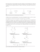
Appendix B: Open/Short Compensation The open/short compensation used in Agilent’s instrument models the residuals of a test fixture or test leads as a linear four-terminal network (a two-terminal pair network) represented by parameters A, B, C, and D (shown in Figure B-1.) This circuit model is basically same as that used in open/short/load compensation. I2 I1 Measurement instrument V1 AB C D V2 Z du t DU T Unknown 4-terminal circuit Figure B-1.
Open measurement When nothing is connected to the measurement terminals (open condition), I2 is 0. Therefore, equation (5) is derived by substituting I2 = 0 for I2 in the equation (2). Here, Zo means the impedance measured with measurement terminals opened. Zo = AV2 A = CV2 C cC = A Zo (5) Short measurement When the measurement terminals are shorted, V2 is 0. Therefore, equation (6) is derived by substituting V2 = 0 for V2 in the equation (2).
Appendix C: Open, Short, and Load Compensation Since a non-symmetrical network circuit is assumed, equation (8) in Appendix B is not applied. Therefore, the relationship between A and D parameters must be determined. The measurement of a reference DUT (load device) is required to determine A and D.
Appendix D: Electrical Length Compensation A test port extension can be modeled using a coaxial transmission line as shown in Figure D-1.
When a (virtual) transmission line in which the signal wavelength is equal to the wavelength in a vacuum is assumed, the virtual line length ( e) that causes the same phase shift (β ) as in the actual line is given by the following equation: λo e = ——— λ 2π 2π e (because β = ———— = —————— ) λ λo Where, λo is a wavelength in vacuum λ is a wavelength in transmission line Therefore, the phase shift quantity, β , can also be expressed by using the phase constant βo in vacuum and the virtual line length e (bec
Appendix E: Q Measurement Accuracy Calculation Q measurement accuracy for auto-balancing bridge type instruments is not specified directly as ±%. Q accuracy should be calculated using the following equation giving the possible Q value tolerance. Qt = 1 1 ± DD Qm Where, Qt is the possible Q value tolerance Qm is measured Q value ΔD is D measurement accuracy For example, when the unknown device is measured by an instrument which has D measurement accuracy of 0.
www.agilent.com www.agilent.com/find/impedance myAgilent myAgilent www.agilent.com/find/myagilent A personalized view into the information most relevant to you. Agilent Channel Partners www.agilent.com/find/channelpartners Get the best of both worlds: Agilent’s measurement expertise and product breadth, combined with channel partner convenience. Three-Year Warranty www.agilent.