Signal Analysis Measurement Guide Agilent Technologies EMC Series Analyzers This guide documents firmware revision A.08.xx This manual provides documentation for the following instruments: E7401A (9 kHz- 1.5 GHz) E7402A (9 kHz - 3.0 GHz) E7403A (9 kHz - 6.7 GHz) E7404A (9 kHz - 13.2 GHz) E7405A (9 kHz - 26.
Notice The information contained in this document is subject to change without notice. Agilent Technologies makes no warranty of any kind with regard to this material, including but not limited to, the implied warranties of merchantability and fitness for a particular purpose. Agilent Technologies shall not be liable for errors contained herein or for incidental or consequential damages in connection with the furnishing, performance, or use of this material.
WARNING This is a Safety Class 1 Product (provided with a protective earth ground incorporated in the power cord). The mains plug shall be inserted only in a socket outlet provided with a protected earth contact. Any interruption of the protective conductor inside or outside of the product is likely to make the product dangerous. Intentional interruption is prohibited. WARNING No operator serviceable parts inside. Refer servicing to qualified personnel. To prevent electrical shock do not remove covers.
LIMITATION OF WARRANTY The foregoing warranty shall not apply to defects resulting from improper or inadequate maintenance by Buyer, Buyer-supplied software or interfacing, unauthorized modification or misuse, operation outside of the environmental specifications for the product, or improper site preparation or maintenance. NO OTHER WARRANTY IS EXPRESSED OR IMPLIED. AGILENT TECHNOLOGIES SPECIFICALLY DISCLAIMS THE IMPLIED WARRANTIES OF MERCHANTABILITY AND FITNESS FOR A PARTICULAR PURPOSE.
Contents 1. Making Basic Measurements What is in This Chapter . . . . . . . . . . . . . . . . . . . . . . . . . . . . . . . . . . . . . . . . . . . . . . . . . . . . . . . . . . . . 8 Test Equipment . . . . . . . . . . . . . . . . . . . . . . . . . . . . . . . . . . . . . . . . . . . . . . . . . . . . . . . . . . . . . . . . 9 Comparing Signals . . . . . . . . . . . . . . . . . . . . . . . . . . . . . . . . . . . . . . . . . . . . . . . . . . . . . . . . . . . . . . . 10 Signal Comparison Example 1: . . .
Contents Tracking Generator Unleveled Condition . . . . . . . . . . . . . . . . . . . . . . . . . . . . . . . . . . . . . . . . . . . . 76 Measuring Device Bandwidth . . . . . . . . . . . . . . . . . . . . . . . . . . . . . . . . . . . . . . . . . . . . . . . . . . . . . 76 Measuring Stop Band Attenuation Using Log Sweep . . . . . . . . . . . . . . . . . . . . . . . . . . . . . . . . . . 79 Making a Reflection Calibration Measurement . . . . . . . . . . . . . . . . . . . . . . . . . . . . . . . . . . . . .
1 Making Basic Measurements 7
Making Basic Measurements What is in This Chapter What is in This Chapter This chapter demonstrates basic analyzer measurements with examples of typical measurements; each measurement focuses on different functions. The measurement procedures covered in this chapter are listed below. • “Comparing Signals” on page 10. • “Resolving Signals of Equal Amplitude” on page 14. • “Resolving Small Signals Hidden by Large Signals” on page 18. • “Making Better Frequency Measurements” on page 22.
Making Basic Measurements What is in This Chapter Test Equipment Test Equipment Specifications Recommended Model 0.25 MHz to 4.
Making Basic Measurements Comparing Signals Comparing Signals Using the analyzer, you can easily compare frequency and amplitude differences between signals, such as radio or television signal spectra. The analyzer delta marker function lets you compare two signals when both appear on the screen at one time or when only one appears on the screen. Signal Comparison Example 1: Measure the differences between two signals on the same display screen. 1.
Making Basic Measurements Comparing Signals Figure 1-1 Placing a Marker on the 10 MHz Signal 9. Press Marker, Delta, to activate a second marker at the position of the first marker. 10. Move the second marker to another signal peak using the front-panel knob, or by pressing Peak Search and then either Next Pk Right or Next Pk Left. Next peak right is shown in Figure 1-2.
Making Basic Measurements Comparing Signals Figure 1-2 Using the Marker Delta Function Signal Comparison Example 2: Measure the frequency and amplitude difference between two signals that do not appear on the screen at one time. (This technique is useful for harmonic distortion tests when narrow span and narrow bandwidth are necessary to measure the low level harmonics.) 1. Perform a factory preset by pressing Preset, Factory Preset (if present). 2.
Making Basic Measurements Comparing Signals 10. Press Marker, Delta to anchor the position of the first marker and activate a second marker. 11. Press FREQUENCY, Center Freq, and the (↑) key to increase the center frequency by 10 MHz. The first marker moves to the left edge of the screen, at the amplitude of the first signal peak. See Figure 1-3. 12. Press Peak Search to place the second marker on the highest signal with the new center frequency setting. See Figure 1-3.
Making Basic Measurements Resolving Signals of Equal Amplitude Resolving Signals of Equal Amplitude Two equal-amplitude input signals that are close in frequency can appear as a single signal trace on the analyzer display. Responding to a single-frequency signal, a swept-tuned analyzer traces out the shape of the selected internal IF (intermediate frequency) filter. As you change the filter bandwidth, you change the width of the displayed response.
Making Basic Measurements Resolving Signals of Equal Amplitude Resolving Signals Example: Resolve two signals of equal amplitude with a frequency separation of 100 kHz. 1. Connect two sources to the analyzer input as shown in Figure 1-4. Figure 1-4 Setup for Obtaining Two Signals 2. Set one source to 300 MHz. Set the frequency of the other source to 300.1 MHz. The amplitude of both signals should be approximately −20 dBm at the output of the bridge. 3. Set the analyzer as follows: a.
Making Basic Measurements Resolving Signals of Equal Amplitude Figure 1-5 Unresolved Signals of Equal Amplitude 4. Since the resolution bandwidth must be less than or equal to the frequency separation of the two signals, a resolution bandwidth of 100 kHz must be used. Change the resolution bandwidth to 100 kHz by pressing BW/Avg, Res BW, 100, kHz. The peak of the signal has become flattened indicating that two signals may be present as shown in Figure 1-6.
Making Basic Measurements Resolving Signals of Equal Amplitude 5. Decrease the video bandwidth to 10 kHz, by pressing Video BW, 10, kHz. Two signals are now visible as shown in Figure 1-7. Use the front-panel knob or step keys to further reduce the resolution bandwidth and better resolve the signals. Figure 1-7 Resolving Signals of Equal Amplitude After Reducing the Video Bandwidth As the resolution bandwidth is decreased, resolution of the individual signals is improved and the sweep time is increased.
Making Basic Measurements Resolving Small Signals Hidden by Large Signals Resolving Small Signals Hidden by Large Signals When dealing with the resolution of signals that are close together and not equal in amplitude, you must consider the shape of the IF filter of the analyzer, as well as its 3 dB bandwidth. (See “Resolving Signals of Equal Amplitude” on page 14 for more information.) The shape of a filter is defined by the selectivity, which is the ratio of the 60 dB bandwidth to the 3 dB bandwidth.
Making Basic Measurements Resolving Small Signals Hidden by Large Signals Resolving Signals Example: Resolve two input signals with a frequency separation of 155 kHz and an amplitude separation of 60 dB. 1. Connect two sources to the analyzer input as shown in Figure 1-9. Figure 1-9 Setup for Obtaining Two Signals 2. Set one source to 300 MHz at −10 dBm. 3. Set the second source to 300.155 MHz, so that the signal is 155 kHz higher than the first signal.
Making Basic Measurements Resolving Small Signals Hidden by Large Signals 5. Set the 300 MHz signal to the reference level by pressing Mkr → and then Mkr → Ref Lvl. If a 10 kHz filter with a typical shape factor of 15:1 is used, the filter will have a bandwidth of 150 kHz at the 60 dB point. The half-bandwidth (75 kHz) is narrower than the frequency separation, so the input signals will be resolved. See Figure 1-10. Figure 1-10 Signal Resolution with a 10 kHz Resolution Bandwidth 6.
Making Basic Measurements Resolving Small Signals Hidden by Large Signals 7. Set the resolution bandwidth to 30 kHz by pressing BW/Avg, Res BW, 30, kHz. When a 30 kHz filter is used, the 60 dB bandwidth could be as wide as 450 kHz. Since the half-bandwidth (225 kHz) is wider than the frequency separation, the signals most likely will not be resolved. See Figure 1-12. (In this example, we used the 60 dB bandwidth value.
Making Basic Measurements Making Better Frequency Measurements Making Better Frequency Measurements A built-in frequency counter increases the resolution and accuracy of the frequency readout. When using this function, if the ratio of the resolution bandwidth to the span is too small (less than 0.002), the Marker Count: Widen Res BW message appears on the display. It indicates that the resolution bandwidth is too narrow.
Making Basic Measurements Making Better Frequency Measurements NOTE Marker count properly functions only on CW signals or discrete spectral components. The marker must be >26 dB above the noise. 9. Increase the counter resolution by pressing Resolution and then entering the desired resolution using the step keys or the numbers keypad. For example, press 10, Hz. The marker counter readout is in the upper-right corner of the screen. The resolution can be set from 1 Hz to 100 kHz. 10.
Making Basic Measurements Decreasing the Frequency Span Around the Signal Decreasing the Frequency Span Around the Signal Using the analyzer signal track function, you can quickly decrease the span while keeping the signal at center frequency. This is a fast way to take a closer look at the area around the signal to identify signals that would otherwise not be resolved. Decreasing the Frequency Span Example: Examine a signal in a 200 kHz span. 1.
Making Basic Measurements Decreasing the Frequency Span Around the Signal Figure 1-14 Detected Signal 8. Turn on the frequency tracking function by press FREQUENCY and Signal Track and the signal will move to the center of the screen, if it is not already positioned there. See figure Figure 1-15. (Note that the marker must be on the signal before turning signal track on.
Making Basic Measurements Decreasing the Frequency Span Around the Signal 9. Reduce span and resolution bandwidth to zoom in on the marked signal by pressing SPAN, Span, 200, kHz. If the span change is large enough, span will decrease in steps as automatic zoom is completed. See Figure 1-16. You can also use the front-panel knob or step keys to decrease the span and resolution bandwidth values. 10. Press FREQUENCY, Signal Track (so that Off is underlined) to turn off the signal track function.
Making Basic Measurements Tracking Drifting Signals Tracking Drifting Signals The signal track function is useful for tracking drifting signals that drift relatively slowly. To place a marker on the signal you wish to track, use Peak Search. Pressing FREQUENCY, Signal Track (On) will bring that signal to the center frequency of the graticule and adjust the center frequency every sweep to bring the selected signal back to the center.
Making Basic Measurements Tracking Drifting Signals Figure 1-17 Signal With Default Span 4. Press Peak Search. 5. Set the span to 10 MHz by pressing SPAN, Span, 10, MHz. See Figure 1-18. Figure 1-18 Signal With 10 MHz Span 6. Press SPAN, Span Zoom, 500, kHz. Notice that the signal has been held in the center of the display. See Figure 1-19.
Making Basic Measurements Tracking Drifting Signals Figure 1-19 Signal With 500 kHz Span 7. Tune the frequency of the signal generator in 10 kHz increments. Notice that the center frequency of the analyzer also changes in 10 kHz increments, centering the signal with each increment. See Figure 1-20. Note that the center frequency has changed.
Making Basic Measurements Tracking Drifting Signals 8. The signal frequency drift can be read from the screen if both the signal track and marker delta functions are active. Set the analyzer and signal generator as follows: a. Press Marker, Delta. b. Tune the frequency of the signal generator. The marker readout indicates the change in frequency and amplitude as the signal drifts. See Figure 1-21.
Making Basic Measurements Tracking Drifting Signals d. Set the center frequency to 300 MHz by pressing FREQUENCY, Center Freq, 300, MHz. See Figure 1-22. Figure 1-22 Signal With Default Span 4. Press Peak Search. 5. Set the span to 10 MHz by pressing SPAN, Span, 10, MHz. See Figure 1-23.
Making Basic Measurements Tracking Drifting Signals 6. Press SPAN, Span Zoom, 500, kHz. Notice that the signal has been held in the center of the display. See Figure 1-24. Figure 1-24 Signal With 500 KHz Span 7. Turn off the signal track function by pressing FREQUENCY, Signal Track (Off). 8. To measure the excursion of the signal, press Trace/View, Max Hold. As the signal varies, maximum hold maintains the maximum responses of the input signal.
Making Basic Measurements Tracking Drifting Signals Figure 1-25 Viewing a Drifting Signal With Max Hold and Clear Write Chapter 1 33
Making Basic Measurements Measuring Low Level Signals Measuring Low Level Signals The ability of the analyzer to measure low level signals is limited by the noise generated inside the analyzer. A signal may be masked by the noise floor so that it is not visible. This sensitivity to low level signals is affected by the measurement setup. The analyzer input attenuator and bandwidth settings affect the sensitivity by changing the signal-to-noise ratio.
Making Basic Measurements Measuring Low Level Signals 10. Reduce the span to 1 MHz. Press SPAN, Span, and then use the step-down key (↓) until the span is set to 1 MHz. See Figure 1-26. Figure 1-26 Low-Level Signal 11. Press AMPLITUDE, Attenuation. Press the step-up key (↑) to select 20 dB attenuation. Increasing the attenuation moves the noise floor closer to the signal.
Making Basic Measurements Measuring Low Level Signals 12. To see the signal more clearly, enter 0 dB. Zero decibels of attenuation makes the signal more visible. See Figure 1-28. Figure 1-28 CAUTION Using 0 dB Attenuation Before connecting other signals to the analyzer input, increase the RF attenuation to protect the analyzer input: press Attenuation so that Auto is underlined or press Auto Couple.
Making Basic Measurements Measuring Low Level Signals 9. Place the signal at center frequency by pressing Peak Search, Marker→, Mkr→CF. 10. Press BW/Avg, Res BW , and then ↓. The low level signal appears more clearly because the noise level is reduced. As shown in Figure 1-29. A # mark appears next to the Res BW annotation at the lower left corner of the screen, indicating that the resolution bandwidth is uncoupled.
Making Basic Measurements Measuring Low Level Signals 3. On the analyzer, perform a factory preset by pressing Preset, Factory Preset (if present). 4. Set the center frequency of the analyzer to 300 MHz by pressing FREQUENCY, Center Freq, 300, MHz. 5. Set the span to 5 MHz by pressing SPAN, Span, 5, MHz. 6. Set the resolution bandwidth to spectrum analyzer coupling by pressing BW/Avg, Res BW (SA). 7. Set the Y-Axis Units to dBm by pressing AMPLITUDE, More, Y-Axis Units, dBm. 8.
Making Basic Measurements Measuring Low Level Signals NOTE Figure 1-31 The video bandwidth must be set wider than the resolution bandwidth when measuring impulse noise levels. Decreasing Video Bandwidth Measuring Low Level Signals Example 4: If a signal level is very close to the noise floor, video averaging is another way to make the signal more visible.
Making Basic Measurements Measuring Low Level Signals 1. Connect a signal generator to the analyzer input. 2. Set the signal generator frequency to 300 MHz with an amplitude of −80 dBm. 3. On the analyzer, perform a factory preset by pressing Preset, Factory Preset (if present). 4. Set the center frequency of the analyzer to 300 MHz by pressing FREQUENCY, Center Freq, 300, MHz. 5. Set the span to 5 MHz by pressing SPAN, Span, 5, MHz. 6.
Making Basic Measurements Measuring Low Level Signals 11. To set the number of samples, use the numeric keypad. For example, press Average (On), 25, Enter. As shown in Figure 1-33. During averaging, the current sample number appears at the left side of the graticule. The number of samples equals the number of sweeps in the averaging routine. Changes in active function settings, such as the center frequency or reference level, will restart the sampling.
Making Basic Measurements Identifying Distortion Products Identifying Distortion Products Distortion from the Analyzer High level input signals may cause analyzer distortion products that could mask the real distortion measured on the input signal. Using trace 2 and the RF attenuator, you can determine which signals, if any, are internally generated distortion products.
Making Basic Measurements Identifying Distortion Products Figure 1-34 Harmonic Distortion 8. Change the center frequency to the value of one of the observed harmonics by pressing Peak Search, Next Peak, Marker→, Mkr→CF. 9. Change the span to 50 MHz: press SPAN , Span, 50, MHz. 10. Ensure that the signal is still at the center frequency, if necessary press Peak Search, Marker→, Mkr→CF. 11. Change the attenuation to 0 dB: press AMPLITUDE, Attenuation, 0, dBm . Your display should be similar to Figure 1-35.
Making Basic Measurements Identifying Distortion Products 12. To determine whether the harmonic distortion products are generated by the analyzer, first save the screen data in trace 2 as follows: a. Press Trace/View, Trace (2), then Clear Write. b. Allow the trace to update (two sweeps) and press Trace/View, View, Marker, Delta. The analyzer display shows the stored data in trace 2 and the measured data in trace 1. 13.
Making Basic Measurements Identifying Distortion Products Figure 1-37 No Harmonic Distortion Third-Order Intermodulation Distortion Two-tone, third-order intermodulation distortion is a common test in communication systems. When two signals are present in a non-linear system, they can interact and create third-order intermodulation distortion products that are located close to the original signals. These distortion products are generated by system components such as amplifiers and mixers.
Making Basic Measurements Identifying Distortion Products Figure 1-38 NOTE Third-Order Intermodulation Equipment Setup The combiner should have a high degree of isolation between the two input ports so the sources do not intermodulate. 2. Set one source (signal generator) to 300 MHz and the other source to 301 MHz, for a frequency separation of 1 MHz. Set the sources equal in amplitude as measured by the analyzer (in this example, they are set to −5 dBm). 3.
Making Basic Measurements Identifying Distortion Products The analyzer automatically sets the attenuation so that a signal at the reference level will be a maximum of −30 dBm at the input mixer. 10. Press BW/Avg, Res BW, and then use the step-down key (↓) to reduce the resolution bandwidth until the distortion products are visible. 11. To measure a distortion product, press Peak Search to place a marker on a source signal. 12.
Making Basic Measurements Identifying Distortion Products Figure 1-40 Measuring the Distortion Product 48 Chapter 1
Making Basic Measurements Measuring Signal-to-Noise Measuring Signal-to-Noise The signal-to-noise measurement procedure below may be adapted to measure any signal in a system if the signal (carrier) is a discrete tone. If the signal in your system is modulated, it will be necessary to modify the procedure to correctly measure the modulated signal level In this example the 50 MHz amplitude reference signal is used as the fundamental source.
Making Basic Measurements Measuring Signal-to-Noise 11. Press More, Function, Marker Noise to view the results of the signal to noise measurement. See Figure 1-41. Figure 1-41 Measuring the Signal-to-Noise Read the signal-to-noise in dB/Hz, that is with the noise value determined for a 1 Hz noise bandwidth. If you wish the noise value for a different bandwidth, decrease the ratio by 10 × log ( BW ) .
Making Basic Measurements Making Noise Measurements Making Noise Measurements There are a variety of ways to measure noise power. The first decision you must make is whether you want to measure noise power at a specific frequency or the total power over a specified frequency range, for example over a channel bandwidth. Noise Measurement Example 1: Using the marker function, Marker Noise, is a simple method to make a measurement at a single frequency.
Making Basic Measurements Making Noise Measurements Figure 1-42 Setting the Attenuation 8. Activate the noise marker by pressing Marker, More, Function, Marker Noise. Note that the display detection automatically changed to “Avg” which can be manually set by pressing Det/Demod, Average (Video/RMS). The marker is floating between the maximum and the minimum of the noise. For firmware revisions earlier than A.08.00, the detection type when using Marker Noise changed to sample.
Making Basic Measurements Making Noise Measurements Figure 1-43 Activating the Noise Marker 9. The noise marker value is based on the mean of 5% of the total number of sweep points centered at the marker. The points averaged span one-half of a division. To see the effect, move the marker to the 50 MHz signal by pressing Marker, 50, MHz (or use the front-panel knob to place marker at 50 MHz). See Figure 1-44. Figure 1-44 Noise Marker at 50 MHz 10.
Making Basic Measurements Making Noise Measurements NOTE Figure 1-45 Notice the video bandwidth changed to 100 kHz. The ratio between the video bandwidth (VBW) and the resolution bandwidth (RBW) must be ≥ 10/1 to maintain the accuracy of the measurement. Increased Resolution Bandwidth 11. Return the resolution bandwidth to 1 kHz. Press BW/Avg, 1, kHz. 12. Measure the noise very close to the signal by pressing Marker, 50.0000, MHz (or use the front-panel knob to place the marker). See Figure 1-46.
Making Basic Measurements Making Noise Measurements Figure 1-46 Noise Marker in Signal Skirt 13. Set the analyzer to zero span at the marker frequency by pressing Mkr →, Mkr → CF, SPAN, Zero Span, Marker. Note that the marker amplitude value is now correct since all points averaged are at the same frequency and not influenced by the shape of the bandwidth filter. See Figure 1-47.
Making Basic Measurements Making Noise Measurements Noise Measurement Example 2: The Normal marker can also be used to make a single frequency measurement as described in the previous example, again using video filtering or averaging to obtain a reasonably stable measurement. While video averaging automatically selects the sample display detection mode, video filtering does not.
Making Basic Measurements Making Noise Measurements 10. Measure the power between markers by pressing Marker, More, Function, Band Power. The analyzer displays the total power between the markers. See Figure 1-48. 11. Add a discrete tone to see the effects of the reading. Turn on the internal 50 MHz amplitude reference signal of the analyzer (if you have not already done so) as follows: • For the E7401A, use the internal 50 MHz amplitude reference signal of the analyzer as the signal being measured.
Making Basic Measurements Making Noise Measurements Figure 1-49 Measuring the Power in the Span 58 Chapter 1
Making Basic Measurements Demodulating AM Signals (Using the Analyzer As a Fixed Tuned Receiver) Demodulating AM Signals (Using the Analyzer As a Fixed Tuned Receiver) The zero span mode can be used to recover amplitude modulation on a carrier signal. The analyzer operates as a fixed-tuned receiver in zero span to provide time domain measurements. Center frequency in the swept-tuned mode becomes the tuned frequency in zero span.
Making Basic Measurements Demodulating AM Signals (Using the Analyzer As a Fixed Tuned Receiver) b. RF Output Power –10 dBm c. AM On d. AM Rate 1 kHz e. AM Depth 80% 2. Set the analyzer as follows: a. Press Preset, Factory Preset (if present). b. Set the center frequency to 300 MHz by pressing FREQUENCY, Center Freq, 300, MHz. c. Set the span to 500 kHz by pressing SPAN, Span, 500, kHz. d. Set the resolution bandwidth to 30 kHz by pressing BW/Avg, Resolution BW, 30, kHz. e.
Making Basic Measurements Demodulating AM Signals (Using the Analyzer As a Fixed Tuned Receiver) 6. Select zero span by either pressing SPAN, 0, Hz; or pressing SPAN, Zero Span. See Figure 1-51. 7. Change the sweep time to 5 ms by pressing Sweep, Sweep Time (Man), 5, ms. 8.
Making Basic Measurements Demodulating AM Signals (Using the Analyzer As a Fixed Tuned Receiver) Figure 1-52 Measuring Modulation In Zero Span Figure 1-53 Measuring Modulation In Zero Span 9. Use markers and delta markers to measure the time parameters of the waveform. a. Press Marker and center the marker on a peak using Peak Search or the front-panel knob. b. Press Marker, Delta and center the marker on the next peak using the front-panel knob or use Peak Search and Next Pk Right (or Next Pk Left).
Making Basic Measurements Demodulating AM Signals (Using the Analyzer As a Fixed Tuned Receiver) Figure 1-54 Measuring Time Parameters 10. You can turn your analyzer into a % AM indicator as follows: a. Set trigger to free run by pressing Trig, Free Run. b. Set the sweep time to 5 seconds by pressing Sweep, Sweep Time, 5, s. c. Set the video filter to 30 Hz by pressing BW/Avg, Video BW , 30, Hz. d.
Making Basic Measurements Demodulating AM Signals (Using the Analyzer As a Fixed Tuned Receiver) Figure 1-55 Continuous Demodulation of an AM Signal 64 Chapter 1
Making Basic Measurements Demodulating FM Signals Demodulating FM Signals As with amplitude modulation (see page 59) you can utilize zero span to demodulate an FM signal. However, unlike the AM case, you cannot simply tune to the carrier frequency and widen the resolution bandwidth.
Making Basic Measurements Demodulating FM Signals 4. Set the span to 1 MHz by pressing SPAN, Span, 1, MHz. 5. Set the Y-Axis Units to dBm by pressing AMPLITUDE, More, Y-Axis Units, dBm. 6. Set the reference level to –20 dBm by pressing AMPLITUDE, Ref Level, –20, dB m. 7. Set the resolution bandwidth to 100 kHz by pressing BW/Avg, Res BW , 100, kHz. The skirt is reasonably linear starting approximately 5 dB below the peak. 8.
Making Basic Measurements Demodulating FM Signals Figure 1-57 Determining the Offset Demodulate the FM Signal 1. Connect an antenna to the analyzer INPUT. 2. Perform a factory preset by pressing Preset, Factory Preset (if present). 3. Tune the analyzer to a peak the peak of one of your local FM broadcast signals, for example 97.7 MHz by pressing FREQUENCY, Center Freq, 97.7, MHz. 4. Set the span to 1 MHz by pressing SPAN, Span, 1, MHz. 5.
Making Basic Measurements Demodulating FM Signals 12. Activate single sweep by pressing Single. See Figure 1-58.
2 Making Complex Measurements 69
Making Complex Measurements What’s in This Chapter What’s in This Chapter This chapter provides information for making complex measurements. The procedures covered in this chapter are listed below. • “Making Stimulus Response Measurements” on page 71. • “Making a Reflection Calibration Measurement” on page 84. • “Demodulating and Listening to an AM Signal” on page 88. To find descriptions of specific analyzer functions refer to the Agilent Technologies EMC Series Analyzers User’s Guide.
Making Complex Measurements Making Stimulus Response Measurements Making Stimulus Response Measurements What Are Stimulus Response Measurements? Stimulus response measurements require a source to stimulate a device under test (DUT), a receiver to analyze the frequency response characteristics of the DUT, and, for return loss measurements, a directional coupler or bridge. Characterization of a DUT can be made in terms of its transmission or reflection parameters.
Making Complex Measurements Making Stimulus Response Measurements Figure 2-1 Transmission Measurement Test Setup 2. Perform a factory preset by pressing Preset, Factory Preset (if present). 3. Set the Y-Axis Units to dBm by pressing AMPLITUDE, More, Y-Axis Units, dBm. 4. Since we are only interested in the rejection of the bandpass filter, tune the analyzer center frequency and span to center the bandpass response and display the rejection ±50 MHz from the center of the bandpass. a.
Making Complex Measurements Making Stimulus Response Measurements Figure 2-2 Tracking Generator Output Power Activated 7. Put the sweep time of the analyzer into stimulus response auto coupled mode by pressing Sweep, Swp Coupling (SR). Auto coupled sweep times are usually much faster for stimulus response measurements than they are for spectrum analyzer (SA) measurements. If necessary, adjust the reference level to place the signal on screen.
Making Complex Measurements Making Stimulus Response Measurements Figure 2-3 Decrease the Resolution Bandwidth to Improve Sensitivity 10.You might notice a decrease in the displayed amplitude as the resolution bandwidth is decreased, (if the analyzer is an E7402A, E7403A, E7404A, or E7405A). This indicates the need for performing a tracking peak. Press Source, Tracking Peak. The amplitude should return to that which was displayed prior to the decrease in resolution bandwidth. 11.
Making Complex Measurements Making Stimulus Response Measurements 12.Reconnect the DUT to the analyzer. Note that the units of the reference level have changed to dB, indicating that this is now a relative measurement. Press Trace/View, More, Normalize, Norm Ref Posn to change the normalized reference position.
Making Complex Measurements Making Stimulus Response Measurements Tracking Generator Unleveled Condition When using the tracking generator, the message TG unleveled may appear. The TG unleveled message indicates that the tracking generator source power (Source, Amplitude) could not be maintained at the selected level during some portion of the sweep. If the unleveled condition exists at the beginning of the sweep, the message will be displayed immediately.
Making Complex Measurements Making Stimulus Response Measurements Measurements are made continuously, updating at the end of each sweep. This allows you to make adjustments and see changes as they happen. The single sweep mode can also be used, providing time to study or record the data. The N dB bandwidth measurement error is typically ±1% of the span. Example: Measure the 3 dB bandwidth of a 200 MHz bandpass filter. 1.
Making Complex Measurements Making Stimulus Response Measurements NOTE To reduce ripples caused by source return loss, use 10 dB (E7401A) or 8 dB (all other models) or greater tracking generator output attenuation. Tracking generator output attenuation is normally a function of the source power selected. However, the output attenuation may be controlled in the Source menu.
Making Complex Measurements Making Stimulus Response Measurements 11.The knob or the data entry keys can be used to change the N dB value from −3 dB to −60 dB to measure the 60 dB bandwidth of the filter. See Figure 2-7. Figure 2-7 N dB Bandwidth Measurement at –60 dB 12.Press N dB Points (Off) to turn the measurement off. Measuring Stop Band Attenuation Using Log Sweep When measuring filter characteristics, it is useful to look at the stimulus response over a wide frequency range.
Making Complex Measurements Making Stimulus Response Measurements Figure 2-8 Transmission Measurement Test Setup 2. Perform a factory preset by pressing Preset, Factory Preset (if present). 3. Set the Y-Axis Units to dBm by pressing AMPLITUDE, More, Y-Axis Units, dBm. 4. Set the start frequency to 100 kHz by pressing FREQUENCY, Start Freq, 100, kHz. 5. Set the stop frequency to 1 GHz by pressing Stop Freq, 1, GHz. 6. Set the resolution bandwidth to 10 kHz by pressing BW/Avg, Res BW, 10, kHz. 7.
Making Complex Measurements Making Stimulus Response Measurements Figure 2-9 Tracking Generator Output Power Activated in Log Sweep 10.Put the sweep time of the analyzer into stimulus response auto coupled mode by pressing Sweep, then Swp Coupling (SR). See Figure 2-9. Auto coupled sweep times are usually much faster for stimulus response measurements than they are for spectrum analyzer (SA) measurements. Adjust the reference level if necessary to place the signal on screen. 11.
Making Complex Measurements Making Stimulus Response Measurements Figure 2-10 Normalized Trace After Reconnecting DUT 14.Press Marker, Delta Pair (Ref), 10, MHz to place the reference marker at the specified cutoff frequency. 15.Press Delta Pair (∆), 20, MHz to place the second marker at the 20 MHz point. In this example, the attenuation over this frequency range is 63.32 dB/octave (one octave above the cutoff frequency). Figure 2-11 Determining Low Pass Filter Rolloff 16.
Making Complex Measurements Making Stimulus Response Measurements Figure 2-12 Minimum Stop Band Attenuation Chapter 2 83
Making Complex Measurements Making a Reflection Calibration Measurement Making a Reflection Calibration Measurement The calibration standard for reflection measurements is usually a short circuit connected at the reference plane (the point at which the device under test (DUT) will be connected.) See Figure 2-13. A short circuit has a reflection coefficient of 1 (0 dB return loss). It reflects all incident power and provides a convenient 0 dB reference.
Making Complex Measurements Making a Reflection Calibration Measurement Reflection Calibration 1. Connect the DUT to the directional bridge or coupler as shown in Figure 2-13. Terminate the unconnected port of the DUT. NOTE If possible, use a coupler or bridge with the correct test port connector for both calibrating and measuring. Any adapter between the test port and DUT degrades coupler/bridge directivity and system source match.
Making Complex Measurements Making a Reflection Calibration Measurement Figure 2-14 Short Circuit Normalized Measuring the Return Loss 1. After calibrating the system with the above procedure, reconnect the filter in place of the short circuit without changing any analyzer settings. 2. Use the marker to read return loss. Press Marker and position the marker with the knob to read the return loss at that frequency.
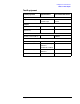
Making Complex Measurements Making a Reflection Calibration Measurement Converting Return Loss to VSWR Return loss can be expressed as a voltage standing wave ratio (VSWR) value using the following table or formula: Table 2-1 Return Loss (dB) Power to VSWR Conversion VSWR Return Loss (dB) VSWR Return Loss (dB) VSWR Return Loss (dB) VSWR Return Loss (dB) VSWR 4.0 4.42 14.0 1.50 18.0 1.29 28.0 1.08 38.0 1.03 6.0 3.01 14.2 1.48 18.5 1.27 28.5 1.08 38.5 1.02 8.0 2.32 14.4 1.
Making Complex Measurements Demodulating and Listening to an AM Signal Demodulating and Listening to an AM Signal The functions listed in the menu under Det/Demod allow you to demodulate and hear signal information displayed on the analyzer. Simply place a marker on a signal of interest, activate AM demodulation, turn the speaker on, and then listen. Demodulating and Listening to an AM Signal Example 1: 1. Connect an antenna to the analyzer input. 2.
Making Complex Measurements Demodulating and Listening to an AM Signal 7. The signal is demodulated at the marker position only for the duration of the demod time. Use the step keys, knob, or numeric keypad to change the dwell time. For example, press the step up key (↑) to increase the dwell time to 2 seconds. 8. The marker search functions can be used to move the marker to other signals of interest. Press Peak Search to access Next Peak, Next Pk Right, or Next Pk Left.
Making Complex Measurements Demodulating and Listening to an AM Signal 11.Press Det/Demod, Detector, Sample to set the detector mode of the analyzer to Sample. 12.Press Det/Demod, Demod, AM. Use the front panel volume knob to control the speaker volume. 13.You can turn your analyzer into a % AM indicator as follows: a. Set trigger to free run by pressing Trig, Free Run. b. Set the sweep time to 5 seconds by pressing Sweep, Sweep Time, 5, s. c.
Making Complex Measurements Demodulating and Listening to an AM Signal Figure 2-17 Continuous Demodulation of an AM Signal Chapter 2 91
Making Complex Measurements Demodulating and Listening to an AM Signal 92 Chapter 2