September 10, 2014 WinLTP Manual Version, 2.10 by William W. Anderson, Ph.D. WinLTP Ltd. support@winltp.com and School of Physiology and Pharmacology University of Bristol Bristol BS8 1TD, England w.w.anderson@bristol.ac.uk Tel: 0117-331-3054 Copyright © WinLTP Ltd. and The University of Bristol, 1991-2014. All Rights Reserved. William W. Anderson asserts his right to be identified as the author of this manual and the WinLTP program under the UK Copyright, Designs and Patents Act of 1988.
1 Table of Contents TABLE OF CONTENTS............................................................................................................................. 1 CHAPTER 1 – INTRODUCTION ............................................................................................................... 5 1.1 WinLTP Capabilities ....................................................................................................................... 5 1.2 Appropriate Equipment....................................
2 4.11 4.12 4.13 4.14 4.15 4.16 4.17 4.18 4.19 4.20 4.21 Setting the Calculation Detection Criteria .................................................................................. 100 Analyzing All S0- and S1-Evoked Postsynaptic Responses in Both AD channels in a Sweep ... 115 Special Analyses of Trains ........................................................................................................ 118 Saving the Protocol File to Disk .............................................................
3 11.5 Printing P0 and P1 sweeps is not necessary for Evoked RepeatSweep stimulation ................. 221 11.6 Evoked Single Sweep stimulation is always shown .................................................................. 223 11.7 Manually Add Events (enter Solution Changes) ....................................................................... 224 11.8 Printing SealTest protocol values ............................................................................................. 227 11.
4 C.5 C.6 C.7 C.8 ‘Reanalyze Again’ Button has been added ................................................................................ 276 Minor Improvements .................................................................................................................. 276 Changes to Basic Version, New Standard Version, WinLTP Now Sold in Units of 1 .................. 276 Bug fixes........................................................................................................................
5 CHAPTER 1 – Introduction 1.1 WinLTP Capabilities WinLTP is a stimulation, data acquisition and on-line analysis program for studying Long-Term Potentiation (LTP), Long-Term Depression (LTD) and other synaptic events such as epileptiform bursts. WinLTP records synaptic activity in extracellular, current-clamp or voltage-clamp modes (at up to 40 KHz/channel).
6 8. On and off-line calculation and plotting of several waveform parameters including: a. DC Baseline b. Peak Amplitude c. Latency d. Slope and Maximum Slope e. Area f. Duration g. Rise Time h. Decay Time i. Coastline j. PopSpike Amplitude k. PopSpike Latency l. Average Amplitude m. Cell Input Resistance (Rm) n. Patch Electrode Series Resistance (Rs) 9. Analyze all S0- and S1-evoked postsynaptic responses in both AD channels in a sweep 10. Special analyses of trains including: a.
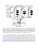
7 toDisk Plot Acquire Stim Sweep toDisk Plot Spont Event In Thread Analyze Continuous Acq In Thread Load Sweep Stimulation Stim Sweep In Thread Continuous Out Thread User Interface Thread Analyze toDisk Plot Detect & Capture Spont Event Output Stimulation Stream M-Series 62xx or Digidata 132x Analog & Digital Out Input Acquisition Stream ‘Revolving Door’ Analog In Fig. 1.1.1.
8 1.2 Appropriate Equipment 1.2.1 Data Acquisition Boards WinLTP currently uses the Axon Digidata 132x boards (the 1320A and 1322A), National Instruments MSeries PCI, PCIe (PCIexpress) and USB 2.0 boards, and also the newer National Instruments X-Series PCIe and USB 2.0 boards. Importantly, the M- and X-Series boards have a 0.5 sec keyboard response delay (compared to 5.0 sec for the Digidata 132x boards). If you are planning to use an National Instruments M- or X-Series board, see Section 2.
9 1.2.2.3 Processor and Speed For National Instruments M- and X-Series boards, WinLTP requires at least a computer with a 2.8 GHz Intel Pentium 4 or higher speed processor with HyperThreading, the faster the better. (Note: some 2.93 and 3.06 GHz Pentium 4 processors do not have HyperThreading, and will not work with the M- or XSeries boards.) For Axon Digidata 132x boards, WinLTP prefers a computer with at least a 3 GHz or higher processor.
10 Put the computer to sleep [30 minutes] change to -> [Never] Note that the automatic turning off of the display does NOT cause problems. For the Axon Digidata 132x board, WinLTP requires the Windows 2000, XP, 7 or 8 (32-bit only) operating system. Note that Windows XP security support from Microsoft has stopped on April 8. 2014, and Microsoft no longer supplies Windows XP security code updates. Therefore, all Windows XP computers should be disconnected from the Internet at this time.
11 Fig. 1.3.1. WinLTP layout for a basic LTP/LTD experiment showing the Protocol fields (upper left panel), analysis graphs (in this case only one slope graph, top right panel), Sweep Acquisition (middle right panel), Sweep Stimulation fields and graphs (lower left and right panels), and the Spreadsheet and Run Buttons (bottom panels). Detection fields to change synaptic potential detection values are hidden behind.
12 The induction of LTP by S0 stimulation (indicated by 'LTP' and up arrow below red triangles in the right top panel of Fig 1.3.1) is produced by evoking by clicking the ‘Single T0’ Run Button which produces a single Train Sweep of 100 S0 pulses at 100 Hz (not shown). The induction of LTD by S0 stimulation (indicated by 'LTD' below red triangles in the top panel of Fig. 1.3.
13 1.6 Conditions of Use CONDITIONS FOR USING WinLTP At the sole discretion WinLTP Ltd., academic users can freely run WinLTP Acquisition in the Basic Mode. However, if academic users wish to run WinLTP Acquisition in the Standard or Advanced Mode after the initial Demotrial period, they must purchase a Standard or Advanced Version license.
14 ADDITIONAL WARRANTY AND LIMITATIONS FOR USING THIS WINLTP SOFTWARE IN THE STANDARD AND ADVANCED MODES 1. Warranty and Liability a. For users running WinLTP Acquisition in the Standard or Advanced Mode using a purchased Standard or Advanced Version license, the maximum liability to WinLTP Ltd. is the cost of the WinLTP Standard or Advanced Version license purchased. 2. Sale of Standard and Advanced Version Licenses a. At the sole discretion WinLTP Ltd.
15 Anderson WW and Collingridge GL (2007) Capabilities of the WinLTP data acquisition program extending beyond basic LTP experimental functions. J. Neurosci. Meth., 162:346-356. or: Anderson WW, Fitzjohn SM and Collingridge GL (2012) Automated multi-slice extracellular and patchclamp experiments using the WinLTP data acquisition system with automated perfusion control. J. Neurosci. Meth., 207:148-160. (whichever is most appropriate). 3.
16 CHAPTER 2 – Getting Started 2.1 Upgrade notice If you are upgrading from earlier versions of WinLTP, you may have to write new *.pro protocol files. The newer WinLTP program will not load protocol files you made using a previous WinLTP if the protocol file size has changed. However, Note that the WinLTP Reanalysis program can analyze the same ADsweep files make with all earlier versions of WinLTP and also the earlier DOS LTP Program. 2.2 Install WinLTP Install WinLTP by running Install_WinLTP210.exe.
17 1) For researchers who can barely afford a data acquisition board: a) PCIe board (with screw terminals): 1) AD board: PCIe-6321 + Cable: SHC68-68-EPM cable, 1 meter + Connector Block (screw terminals): CB-68LPR 2) Free Basic Version of WinLTP $764 0 --------------------- Total 2) For most researchers: a) PCIe board (with screw terminals): 1) AD board: PCIe-6321 + Cable: SHC68-68-EPM cable, 1 meter + Connector Block (screw terminals): CB-68LPR 2) Standard Version of WinLTP (1st copy is $700, additional
18 2.4 Install the National Instrument PCI M- or X-Series board NOTE: The M- and X-Series PCI, PCIe (PCIexpress) and USB 2.0 boards have a 0.5 sec keyboard response delay (compared to 5.0 sec for the Digidata 132x boards). 2.4.1 M- and X-Series Data Acquisition Boards Fairly recently, National Instruments has introduced the X-Series of boards along side the M-Series boards. The X-series boards are slightly higher performance than the M-Series boards.
19 Note that the current 2.10 version of WinLTP samples at 200 kSamples/sec, so there is need to necessarily buy 500 kSamples/sec or 1 MSamples/sec boards. Future versions of WinLTP may utilize 1 MSamples/second capability, but this is not guaranteed.
20 analog outputs and > 8 high-speed digital outputs are not supported with WinLTP 2.10 but will be in subsequent versions – so there is no need to buy the second cable and additional connections now.) You could also use other connector boxes such as the SCB-68 Shielded Connector Box, but there is little point, as it is about the same cost as the others, and only has screw terminal outputs. NOTE: WinLTP 1.10 and earlier was only set to run in the NRSE (Non-Referenced Single-Ended) mode.
21 Fig. 2.4.3.1. Making measurements in Differential, Non-Referenced Single-Ended (NRSE), and Referenced Single-Ended mode (RSE) modes. Use Differential, NRSE or RSE mode to connect a Floating Signal (FS) Source such as a battery powered biological amplifier NOT connected to mains ground. Usually use Differential or NRSE to connect a Grounded Signal (GS) Source such as a biological amplifier connected to mains ground (Copyright National Instruments, 2011). 2.4.3.1 BNC-2110 Connector Box The BNC-2110 (Fig.
22 For a Floating Signal (FS) Source such as a signal from a battery powered biological amplifier, switch the FS/GS switch to FS. For a Ground Signal (GS) Source such as a signal from a mains powered and grounded biological amplifier, switch the FS/GS switch to GS. Analog Outputs 0 and 1 are used as normal (plugged into with a shielded BNC cable). To use the extracellular stimulation outputs, connect a wire from pin P0.0 to User1 (so that the User1 BNC can be S0 output), and connect a wire from pin P0.
23 2.4.3.2 BNC-2090A Connector Box NOTE: In WinLTP 1.10 and earlier, the BNC-2090A was used in NRSE recording mode and required setting the SE/DIFF switches to SI, and the RSE/NRSE to NRSE (Non-Referenced Single Ended). In WinLTP 1.11 onward the recording mode can now be Differential, NRSE or RSE depending what is chosen in the Choose Recording Mode radiobutton group (Fig. 2.8.4). Analog Inputs 0 and 1 (ACH0 and ACH1) are used as normal (plugged into with a shielded BNC cable).
24 How to use the CB-68LPR screw terminal connections (note that the The pinout numbers/functions of the PCIe-6321 (left) are the same pinout numbers/functions in the CB-68LPR (right) (Fig. 2.4.3.3.
25 For connecting the analog outputs: For IC0 (AO0): Center wire of coaxial cable to pin 22 (AO0) Shield wire of coaxial cable to pin 55 (AO Gnd) and possibly also ground to your system ground if necessary For IC1 (AO1): Center wire of coaxial cable to pin 21 (AO1) Shield wire of coaxial cable to pin 54 (AO Gnd) and possibly also ground to your system ground if necessary Fig. 2.4.3.3.1.
26 And either just put the connector in a plastic box (like a simple takeaway box), or if shielding seems necessary a metal box. If you use a metal box you could also use BNCs with the outer connector connected to a separate pin. This is a bit of a pain to install initially (compared the using the BNC 2110), but once its installed you probably don’t really need to change things around much and it should be fine. 2.4.3.4 BNC-2120 Connector Box NOTE: In WinLTP 1.
27 However, future versions of WinLTP will include at least 5 analog inputs, 4 analog outputs, 8 to 24 highspeed digital outputs, and maybe 8 low-speed digitial outputs. For this you can use either two BNC2110’s, two BNC-2120’s, two BNC-2090A’s or using the CA-1000 enclosure (with BNC panelettes and two CB-68LPR connector blocks). So wiring up a CA-1000 is not completely unreasonable. Installation is pretty easy and requires only a supplied screwdriver.
28 Fig. 2.4.4.1. Top) The pinout numbers/functions of the USB-6341 screw terminals and bottom) the connections and pinouts of the USB-6341 BNC board (the chassis ground is in yellow) (Copyright National Instruments, 2013).
29 2.4.5. Install NI-DAQmx 9.x You first have to install NI-DAQmx from the CD included with your M- or X-Series board. For these boards, version 8.8 or higher must be used because of the code added to support USB M-series boards, and version 9.5 or higher must be used to support the X-Series boards. If you need to upgrade, you might as well download and use the latest Version 9.9 from www.ni.com. Follow the installation instructions.
30 can simultaneously run depends on the speed of your computer (it should at least be a dual-core), and the rate at which you run and save sweeps during an experiment (be sure to test beforehand). To install a second M- or X-Series board in your computer perform the following steps: 1) Make sure the WinLTP program that uses the “Dev1” board is not running. 2) Install a second National Instruments M- or X-Series board into your computer.
31 Fig 2.4.7.1. The Set M,X-Series Board Device Number dialog box used to set the Device Number of an additional M- or X-Series board. 2.5 Install the Axon Digidata 1320A or 1322A board 2.5.1 Install Digidata board in Windows 2000 or XP NOTE: If you are installing just the WinLTP Reanalysis program, you do not have to first install AxoScope or pClamp, inotherwords (e.g., you can skip this section). 2.5.1.
32 antivirus/antimalware program will continue to be updated until July, 2015. Rather than upgrade your Windows XP computer, the simplist thing to do is to just disconnect your Windows XP computer from the Internet, and transfer your WinLTP data using a USB memory stick. 2.5.1.
33 2.5.2.1 Install the SCSI card Put the SCSI card into the computer and connect the Digidata 1320A or 1322A board to the SCSI card according to the instructions from Axon Instruments included with the board. Do not power up the board, but turn on the computer to see that the SCSI card is recognized. Molecular Devices has recommended the Tekram DC-395U, the Tekram DC-395UW, and the Adaptec 29160N SCSI cards.
34 Fig 2.6.1. When WinLTP starts up, the initial ‘splash screen’ comes up almost immediately indicating that the program in “Loading…”, which takes at least 15 seconds. After this period the “Loading…” message goes away and the initial Data Root Folder is shown (Fig. 2.7.1). NOTE: There may be a video related BUG with early versions of Windows XP. If WinLTP hangs up during start-up (start-up can take at least 15 seconds!), try changing your video to Classic (Windows 2000) mode.
35 subfolder with today’s data where data will be written) are created as shown in Fig. 2.7.3. You can also change the Data Read/Write Folder while running an experiment (Section 4.16). Fig. 2.7.1. ‘Splash screen’ showing the initial Data Root Folder. This ‘splash screen’ is the one shown if running in the Demotrial Period showing the number of days left, the ending date, and the fact that you can currently run WinLTP in the Advanced Mode.
36 Fig. 2.7.2 The Change Data Root Folder dialog box. Fig. 2.7.3. ‘Splash screen’ showing the final Data Root Folder, and the Data Read/Write Folder into which data will be written during acquisition and analysis.
37 2.8 Choose the Connector Box and Recording Mode for M-,XSeries boards If this is the first time WinLTP has been run on this M or X-Series board, an ‘Edit Protocol (Set M- or XSeries Connector Box and Recording Mode, first time program run)’ dialog box will appear (Fig. 2.8.1). Fig. 2.8.1. The Resources tabsheet in the Edit Protocol (Set M- or X-Series Connector Box and Recording Mode, first time program run)’ dialog box showing the choice of a BNC-2110 Connector Box.
38 settings or pin-to-pin wire connections that need to be made. The bottom lines (if any) give a WARNING (in yellow) for any setting need be changed when upgrading from WinLTP 1.10 or earlier. NOTE: After you have chosen the Connector Box you installed in Section 2.4.3 and have chosen the Recording Mode, set any switches mentioned in the Information Panel, and any pin-to-pin wire connections required.
39 Fig. 2.8.4. The Resources tabsheet in the Edit Protocol (Set M- or X-Series Connector Box and Recording Mode, first time program run)’ dialog box showing the choice of a BNC-2090A Connector Box. With the BNC-2090A you can choose between Differential recording mode (top panel) , Non-Referenced Single-Ended (NRSE) mode (lower left panel), and Referenced Single-Ended (RSE) mode (lower right panel).
40 Fig. 2.8.5. The Resources tabsheet in the Edit Protocol (Set M- or X-Series Connector Box and Recording Mode, first time program run)’ dialog box showing the choice of a connector box with all pins available such as the CA-1000 enclosure with a CB-68LPR connector block. With the connector box with all pins available, you can choose between Differential recording mode (top panel) , Non-Referenced Single-Ended (NRSE) mode (lower left panel), and Referenced Single-Ended (RSE) mode (lower right panel. 2.
41 For M or X-Series boards, National Instruments recommends that the computer and board have warmed up for at least 15 minutes. Also, National Instruments recommends that you periodically self-calibrate the board by clicking on: Options -> Recalibrate Data Acquisition Board Fig. 2.9.1. The Calibrate M-Series dialog box after calibration has successfully concluded. Fig. 2.9.2. The Calibrate Digidata 132x dialog box after calibration has successfully concluded. 2.
42 Help -> Electrode / Data Acquisition Board Connections… to call up the Electrode <-> Acquisiton Board Connections dialog box (Fig. 2.10.1). Fig. 2.10.1. Electrode <-> Acquisition Board Connections dialog box to connect the extracellular stimulation SIUs, recording amplifier analog inputs and outputs, and digital outputs to the Digidata 132x data acquisition board.
43 When WinLTP first starts in the Demotrial Period, a series of ‘Info Slides’ appears (a new one for each day) first describing What’s New in this version of WinLTP (Fig. 2.11.1). After these What’s New slides are shown, then an Info Slide describing the differences between Basic, Standard and Advanced Modes, and why we are now selling it with dongle copy protection (Fig. 2.11.2). This is then followed by an Info Slide that briefly shows what happens after the 60 day Demotrial Period ends (Fig. 2.11.3).
44 Fig. 2.11.2. The second to the last Info Slide briefly describing the differences between Basic, Standard and Advanced Modes, and selling WinLTP in units of 1 with dongle protection. Fig. 2.11.3. The last Info Slide briefly showing what happens after the 60 day Demotrial Period ends.
45 2.11.2 Post-Demotrial Period - Basic Mode If no Temporary or Permanent (Advanced Version) License Key file is installed or no Standard or Advanced Version dongle is connected to your computer, after this 60 day Demotrial Period, WinLTP will automatically run in the Basic Mode. When WinLTP is started at this time, the ‘splash screen’ will display the following message saying when the Demotrial Period ended and that WinLTP is running in the Basic Mode (Fig. 2.11.2.1).
46 2.11.3 Temporary License Key – Advanced Mode A Temporary License Key file can run WinLTP in the Advanced Mode. If there is a reason, WinLTP Ltd. can send you a time-limited Temporary License Key file which you put into the \WinLTP program folder to allow you to temporarily run WinLTP in the Advanced mode. If you are using a Temporary License Key file, you will see the following message at the bottom of the beginning ‘splash screen’ (Fig. 2.11.3.1). Fig. 2.11.3.1.
47 bottom of the beginning ‘splash screen’ (Fig. 2.11.5.2). This tells you that the key is permanent (i.e. timeunlimited), and that you can permanently run WinLTP in the Advanced Mode. Fig. 2.11.4.1. ‘Splash screen’ showing that a Standard Version USB dongle has been detected, and that it was licensed to run on this computer, who and where it was licensed to, and that you are permanently running WinLTP in the Standard Mode. Fig. 2.11.5.1.
48 2.12 Basic, Standard and Advanced Mode Capabilities When you enter the WinLTP program for the first time in the Demotrial period you are running in the Advanced Mode with a fully functioning Protocol builder (Fig. 2.12.1, left) including automated perfusion. In this mode you can write any number of advanced protocols including this automated perfusion protocol using ‘Slow0’ and ‘Slow1 Perfuse’ events.
49 Fig. 2.12.1. The Advanced, Basic and Standard Modes of WinLTP. Left) When you enter the WinLTP program for the first time in the 60 day Demotrial period you are running in the Advanced Mode with a fully functioning Protocol builder including automated perfusion. All the Insert Event buttons can be used and are marked in green. Middle) In the Basic Mode, the Protocol Builder is partially function and only the green Insert Events can be used, not those in yellow.
50 A B C Fig. 2.12.2. Additional capabilities that are present in the Standard and Advanced Versions but absent in the Basic Version. A) The Experimental Log cannot be saved in the Basic Version (indicated by yellow). B) Continuous Acquisition files and channel AD1 for the Acquisition/Stimulation Sweeps cannot be saved in the Basic Version (indicated by yellow).
51 For now just click on the ‘Init’ Protocol button (Fig. 2.12.1, right top panel), to be able to run repetitive P0sweeps. 2.13 Set the AD Gain, DataType, Sample Interval and Other Parameters 2.13.1 Set the AD Gain, Data Type, and Sample Interval in the Edit Protocol dialog box Once in the Edit Protocol dialog box, click on the Acquisition/Stimulation Parameters tabsheet (Fig. 2.13.1.1).
52 First, set the channel AD0 DataType to "mV". Second, change the AD0 Gain to be equal to the total amplification gain from the electrode to the AD board connection. For example, if an Axon Instruments AxoClamp is used in current clamp mode with an internal x10 output gain, which then goes into an external x100 amplifier and then into channel AD0, the AD0 Gain would be 1000.
53 2.14 Analog Filtering of the Signal Before Digitization The waveform signal data should be filtered before being digitized with an analog filter set to half or less of the digitization frequency. For example, if you are acquiring an AD sample at 50 µsec intervals (e.g. at 20 KHz sampling frequency), the analog filter should be set to at maximum 10 kHz (1/2 the sampling frequency), or preferably to 5 kHz or lower (except if doing an Rs exponential fit, then keep it at 10 KHz).
54 Then use the menu command: View -> Select Columns… to call up the Select Columns dialog box and then select CPU Usage, Memory Usage, Peak Memory Usage and any other you want such as, in this example, Base Priority and the number of Threads. Fig. 2.17.1 shows a relatively low CPU usage of about 9% when running WinLTP with a Digidata 1322A board on a 3.
55 Also note the small green CPU Usage Graph on the right of the Task Bar which concisely shows CPU usage as a % full usage. This can be kept on screen all the time to show CPU usage (with the Task Manager minimized). Fig. 2.17.2. Windows Task Manager showing CPU usage graphically after the MainProtocol was started. Note the small green CPU Usage Graph on the right of the Task Bar. Alternatively, CPU usage can also be seen graphically by clicking on the Performance tab (Fig. 2.17.
56 Fig. 2.17.3. Windows Task Manager showing usage of 2 CPUs in a dual-core processor graphically after the MainProtocol was started. 2.18 Ways to speed up WinLTP on slower computers There are a few ways of speeding up WinLTP on slower computers without buying a new computer. Basically, do a dry run of your experimental protocol including all stimulation and saving data to disk before actually running the experiment.
57 (e.g. Fig. 2.17.1), you may find that your anti-virus program may be using half the CPU power to check that the WinLTP files being saved (*.ABF and *.P0 etc. files) do not contain a virus. The chances that they do are practically nil, particularly for the ASCII *.P0 etc. files. If disabling your anti-virus program makes a difference, you can re-enable the On-Access capability of your anti-virus program, but exclude anti-virus scanning of specific file types ABF and P0 etc. with your anti-virus program.
58 CHAPTER 3 – Organization of WinLTP 3.1 Tabsheet and Panel Areas WinLTP is organized in multiple tabsheets and panels. Fig. 3.1.1 shows the basic WinLTP tabsheet and panel layout for a basic LTP experiment.
59 3.1.1 MainPg/AnalysisPg Tabsheet Area The upper right corner of the program shows the MainPg and AnalysisPg tabsheets (Fig. 3.1.1.1).
60 The AnalysisPg contains one or two columns of Analysis graphs with one to four Analysis graphs in each column (however, in this version the AnalysisPg is not implemented). 3.1.2 Link/Protocol/Log/Detect Tabsheet Area The upper left corner of the program shows the Link/Protocol/Log/Detect tabsheet area containing the Link tabsheet (Fig. 9.1.1), the Protocol tabsheet (Fig. 3.1.2.1), the Log tabsheet (Fig. 11.1.1), and the Detect tabsheet (Fig. 3.1.2.3).
61 Advanced Mode Standard Mode Basic Mode Fig. 3.1.2.1. The Protocol tabsheet in the Advanced Mode (including Demotrial Period) fully functional ‘Protocol Builder’ (left), and (with the same protocol) in the Basic Mode partially functional ‘Protocol Builder’ (right). The Link tabsheet is discussed in Chapter 9. The Protocol tabsheet then has four ‘sub’ tabsheets consisting of the Perfuse tabsheet (Fig. 10.2.7.2), the MainProtocol tabsheet (Fig. 3.1.2.1), the Evoked Events tabsheet (Fig. 3.1.2.
62 Fig. 3.1.2.2. The Evoked Tabsheet for the Standard and Advanced Modes (left) with full capability, and for the Basic Mode (right) missing the T1 evoked sweeps.
63 Standard and Advanced Modes Basic Mode Fig. 3.1.2.2. The Plot/Save ‘sub’ tabsheet of the Protocol tabsheet for the Standard and Advanced Modes (left) with full functionality, and in the Basic Mode.. Note that in the Basic Mode, the ‘Cont Acquis’ ‘Save To Disk’ checkboxes are marked in yellow indicating that Continuous Acqusition data cannot be saved in the Basic Mode, and Channel AD1 cannot be saved for the Acquisition/Stimulation Sweeps.
64 Fig. 3.1.2.3.. Detect tabsheet containing both the AD0 and AD1 ‘sub’ tabsheets. 3.1.3 Sweep Stimulation Field Area The middle left area of the program shows the Sweep Stimulation field area, the area where value fields that control stimulation values for each sweep, P0, P1, T0 and T1, are located. For instance, Fig. 3.1.3.1 shows P0 Sweep Stimulation that includes Sweep Duration and S0 Pulse Duration, Interval and Number in the S0 ‘sub’ tabsheet.
65 Fig. 3.1.3.2. IC0 stimulation fields. Note that the Field Sweep Stimulation area is functionally coupled with the Graph Stimulation area, so that when you click on the P0 tabsheet in the Field Sweep Stimulation area, the P0 Sweep Stimulation graph comes up (Fig. 3.1.3.3). And when you click on the T0 tabsheet in the Field Sweep Stimulation area, the T0 Sweep Stimulation graph comes up, and so forth. Fig. 3.1.3.3. Field and Graph Sweep Stimulation Areas are coupled. 3.1.
66 c) Time Of Day (in hr:min:sec) where hr increases to 25 after 24, not 0 d) Time on the Analysis graph the data point was taken (in Min:Sec.
67 Standard and Advanced Modes Basic Mode Fig. 3.1.5.1. Run Panel (left) and Run Buttons (right). The Run Buttons show full functionality for the Standard and Advanced Modes (top), but lack the evoked Single and Repeat T1sweeps for the Basic Mode (bottom). 3.1.6 Status Bar The Status Bar area (Fig. 3.1.6.
68 Fig. 3.2.1. Protocol File Menu Fig. 3.2.2. SweepFile Menu. Fig. 3.2.3. Amplitude File Menu. Fig. 3.2.4. Options Menu (The Set M,X-Series Board Device Number only appears when running the Mor X-Series National Instruments boars).
69 Fig. 3.2.5. View Menu. Fig. 3.2.6. Run Menu. Fig. 3.2.7. Help Menu. 3.3 Running Protocols using Run Buttons, Function Keys and Run Menus Protocols can be started by either clicking a Run Button, pressing a Function Key, or by choosing the correct line in the Run menu (Fig. 3.2.6). The Run menu gives a description of the protocol on the left side of the line, and the shortcut Function Key that can be alternatively pressed to start that protocol.
70 3.4 Fields – Changing Values Fields can be selected by Tabbing or Shift-Tabbing (reverse) into them, and are indicated selected by turning dark blue. Selected field values can be changed by: 1) Entering values using the keyboard and pressing the Enter key 2) Pressing the Left Mouse Button to increment a value, and pressing the Right Mouse Button to decrement a value. 3) Moving the Mouse Thumbwheel forward to increment a value, and moving the Mouse Thumbwheel backwards to decrement a value.
71 b) Or, more simply, for ADsweep graphs you can press the Ctrl-U key, or click the View -> Unzoom menu item. You cannot do this for Analysis graphs. 3) For ADsweep graphs you can also toggle back and forth between the Zoomed and Unzoomed states by pressing either the Ctrl-Z key (or the View -> Restore Previous Zoom menu item) to enter the Zoomed state, or press the Ctrl-U key (or the View -> Unzoom menu item) to enter the Unzoomed state.
72 a b c Fig. 3.5.1. ADsweep graph Zooming and Unzooming. a) Non-Zoomed state. There is no “Unzoomed” label on the lower left axis. The mouse cursor has been dragged from the upper-left to the lower right around the first EPSC (but not released) and this ADsweep graph is about to be zoomed. b) Zoomed state. There is a red “Zoomed” label on the lower left axis.
73 3.6 Coding of Synaptic Waveform Detection Different colors are chosen in the program depending on whether a synaptic potential was stimulated by S0 or S1 stimulation. Red denotes extracellular electrode S0 stimulation in the Train and Pulse Sweep Stimulation panels (Fig. 3.1.3.1). Red marks the superimposed DC Baseline, Peak Amplitude, Slope etc superimposed calculation lines for the first S0 stimulation in the Pulse ADsweep graphs in the Pulse Detection panel (Fig. 3.1.2.
74 CHAPTER 4 – Running a Basic LTP Experiment In the Getting Started section (Chapter 2) an initial configuration of the program has been performed. This includes: 1) Installing WinLTP 2) Installing the data acquisition board. 3) Starting WinLTP 4) Making the appropriate connections to the data acquisition hardware from the recording amplifier and stimulus isolation units (SIUs). 5) Setting up data acquisition and stimulation parameters 6) Acquiring a sweep of data 4.
75 If a custom Protocol File to run your particular experiment has not yet been developed, the following procedures should be performed to fully implement the protocol. Essentially this involves: 1) Choose whether or not to use Continuous Acquisition 2) Writing the script in the Protocol Builder, often to just continuous looping or continuous looping with Signal Averaging 3) Setting up the data acquisition values. 4) Choosing the Stimulation Protocols. 5) Setting Train and Pulse stimulation values.
76 Insert Event buttons can be used and still save ADsweep data. These include ‘AvgLoop’, ‘Loop’, ‘P0sweep’ and P1sweep events. If you use the yellow Insert Event buttons, the ‘Run’, ‘ElseRun’, ‘Tosweep’ ‘T1sweep’ and ‘Delay’ events, your protocol will run perfectly OK, except that the ADsweep data will not be saved. This allows you to easily test the Advanced Mode functions to see if it is worthwhile upgrading to the Advanced Version. 4.4.
77 A B Fig. 4.4.1.1. Writing simple Protocol Builder scripts to do A ) slow Repetitive P0 Pulse Sweeps once every 10 sec (top) and repetitive alternating P0 then P1sweeps every 20 sec. B) Slow Repetitive P0sweeps with signal averaging, and repetitive alternating P0 then P1 sweeps, one averaged P0sweep also every 80 sec. Obviously you would change the period times to something more suitable – 10 sec is the initial sweep period value.
78 Finally, if you want to produce repetitively alternating P0/P1sweeps with signal averaging, again you 1) press down the LeftMouseButton to click on the ‘P1sweep’ Insert button, 2) hold the LeftMouseButton down to drag the P1sweep down to just below the P0sweep in the MainProtocol script, and then 3) release the LeftMouseButton to insert the P1sweep just below the P0sweep (see red line/arrow in Fig. 4.4.1.1B, bottom).
79 4.4.2.1 Enabling Evoked Single Sweep Stimulation The check boxes in the ‘Single Train or Pulse Sweep’ panel in Fig. 4.4.2.1 (top of top panel) determine whether these single sweeps can be evoked by clicking single Run Buttons, Function Keys or Run Menu items (Sections 3.1.5 and 3.3, and Figs. 3.1.5.1 and 3.2.6). Fig. 4.4.2.1 shows a Single T0sweep is enabled and only the ‘Single T0’ button of all the Single Sweep Run Buttons in the bottom panel is enabled and ready to be clicked on. 4.4.2.
80 A B Fig. 4.4.2.2.1. Add one extra Delay period after an LTD stimulation. A) LTD stimulation with no extra Delay period. At the arrow, the ‘Repeat P0’ sweep button was clicked and a 20 pulse LTD stimulation (1 pulse/sweep) started after the last AvgLoop was exited. The 1st post-LTD pulse looked like 21st pulse of LTD stimulation. B) LTD stimulation with one extra Delay period.
81 Function Keys or Run Menu items ((Sections 3.1.5 and 3.3, and Figs. 3.1.5.1 and 3.2.6). These enabling check boxes work the same way as those for the Repeat P0 Sweeps. The first field to the right of the check box determines the number of times a sweep is repeated. The next field to the right is the period of the sweep (in seconds). Finally, the text following the equal sign is the total time of the sweep in min:sec.
82 Fig. 4.4.2.4.1. Evoked Repeat PulseSweeps can not occur in an Average Loop. At arrow, the ‘Repeat P0’ sweep button was clicked evoking the LTD stimulation which only started after 2nd Average Loop exited. Also note that For LTD stimulation with averaging, the current and total number of sweeps evoked is now written on the RunLine. However, evoking Single or Repeat T0 or T1 sweeps in an Averaging Loop is fine because these do not have a sum array and averaging is never done on them.
83 A B Fig. 4.5.1. A) Enable Sweep Functions panel in the MainProtocol tabsheet. B) Save Sweeps To Disk panel in the Plot/Save tabsheet. Single raw sweeps can either be (i) low-pass filtered, (ii) stimulus artifact blanked, or (iii) stimulus artifact blanked and then filtered (Fig. 4.5.2a) (but not first filtered and then stimulus artifact blanked). The insets in Fig. 4.5.
84 Fig. 4.5.2. Raw sweeps can be signal averaged, stimulus artifact blanked, and/or low-pass digitally filtered. a) Raw sweeps (with no signal averaging) can be digitally low-pass filtered, stimulus artifact blanked, or stimulus artifact blanked first and then filtered. The insets show the raw sweep (left trace), the filtered sweep (right top trace), the stimulus artifact blanked sweep (middle trace), and the blanked and filtered sweep (right bottom trace).
85 4.5.1 Signal Averaging If Signal Averaging is used, each sweep is first acquired and plotted in Gray, then the average of the sweeps is then plotted in LightBlue. The setting for the number of sweeps to average for the Slow Repeat Sweeps is set by the AvgLoop number of loops field - see Fig. 3.1.2.1 for a simple averaging protocol, and Figs. 7.4.1.1, 7.4.9.1 and 7.4.10.1 for more complex averaging protocols.
86 a Average b Slope c Hold Fig. 4.5.2.1. The a) Average, b) Slope and c) Hold methods of blocking stimulus artifacts.
87 4.5.4 Low-Pass Digital Filtering Low-pass digital filtering is done using a Gaussian digital filter (Colquhoun D, and Sigworth, FJ, Fitting and statistical analysis of single channel records. In B. Sakmann and E. Neher editors. Single Channel Recording. Plenum Press, London, 191-263, 1983). If Low-Pass Filtering is chosen, each sweep is first acquired and plotted in Gray, and then digitally filtered at an appropriate frequency and plotted in LightBlue.
88 4.5.4 Erase Raw, Averaged, Blanked Traces if Low-Pass Filtering If you are using an amplifier which does not have low-pass filtering to record your synaptic activity (such as several intracellular amplifiers), there is no low-pass filtering to remove excess noise that is necessary for correct analysis of many parameters such as peak amplitude.
89 Fig. 4.5.4.1. Using the “Erase Raw/Averaged/Blanked Traces if Filtering” check box to remove the unnecessary raw trace when doing low-pass digital filtering. The top panel shows the raw (gray) trace and 1000 Hz low-pass filtered (blue) trace when the “Low-Pass Filtering” check box is checked, and the “Erase Raw/Averaged/Blanked Traces if Filtering” check box (red arrow) is unchecked.
90 4.6 Setting Which Sweeps to Save to disk The ‘Save Sweeps To Disk’ panel (Fig. 4.6.1) in the Plot/Save tabsheet (Fig. 4.5.1B, also see Fig. 3.1.2.2, right) sets which sweeps will be saved: 1) Raw Sweeps enables saving raw Pulse, Train or Spontaneous Sweeps to disk 2) Averaged Sweeps enables saving only averaged Pulse Sweeps to disk (Trains Sweeps, because they cannot be averaged, cannot be saved as averaged sweeps).
91 Fig. 4.7.1. AD Channels to Plot and Save Panel. Then check which AD channels you want to plot for Continuous Acquisition and Stimulation Sweeps, and which AD channels you want to save to disk for Continuous Acquisition and Stimulation Sweeps. Note that Plotting and saving to Spontaneous Sweeps is currently disabled. 4.8 Set the Data Acquisition Values Setting Analog Input values has already been discussed in Section 2.13.1. 4.8.
92 4.9 Choosing Pulse/Train Sweep Stimulation Protocols and Setting Stimulation Values The complete stimulation output of WinLTP is a combination of the output of the P0, P1, T0 and T1sweeps in the Protocol Builder (Chapters 7, 8 and 10) plus the Evoked Single and Repeat Sweeps. 4.9.1 Choosing the Sweep Stimulation Protocol The extracellular, intracellular and digital stimulation in each sweep is controlled by the fields in the P0, P1, T0 or T1 tabsheet in the Sweep Stimulation area (Fig. 4.9.1.
93 Then choose whether you want to change S0 extracellular stimulation, S1 extracellular stimulation or Intracellular analog channel 0 (and possibly digital) stimulation by clicking on the S0, S1 or IC0 tabsheet. S0 and S1 stimulation can be either ‘Off’ or ‘On’ as set by the pop-up menu that pops up when the mouse cursor is clicked on the S0 or S1 Label/Button in the S0 or S1 tabsheet (Fig. 4.9.1.2). Fig. 4.9.1.2.
94 Fig. 4.9.1.3. Setting S0 output to ‘Pulses’ or ‘Trains’ by clicking on the Pulses/TrainsB Label/Button that raises up when the mouse cursor is moved over it. IC0 stimulation can be either ‘Off’, ‘Amplitude’ On, or ‘Amplitude + Digital Out’ On as set by the pop-up menu that pops up when the mouse cursor is clicked on the S0 or S1 Label/Button in the S0 or S1 tabsheet (Fig. 4.9.1.4). Fig. 4.9.1.4.
95 Note that Epoch0 only can go to ‘Off’, ‘Step’ or ‘Begin Loop’, not ‘RsRm Step’, ‘Ramp’ or ‘EndLoop’ because there is no previous step with which to use in the Rs/Rm measurements, you need a Step before a Ramp to set the initial amplitude, and a loop cannot begin on an EndLoop. Fig. 4.9.1.5.
96 Fig. 4.9.2.1. Heterosynaptic paired-pulse stimulation can help test for pathway independence. Theta burst stimulation in a single sweep. Fig. 4.9.2.2 shows a theta burst stimulation in a single sweep (rather than single trains in repeating sweeps) capable of inducing LTP. S0 Epoch B is set to Trains, and the NumTrains is set to greater than 1 to get repetitive train stimulation. Fig. 4.9.2.2. Theta burst stimulation for LTP induction consisting of repeating trains in a single sweep.
97 Fig. 4.9.2.3. Primed burst stimulation for LTP induction consisting of a single pulse on one digital output (D2), and a single train on another digital output (S0) which then go to trigger the same Stimulus Isolation Unit by using an OR chip or two diodes. Fig. 4.9.2.4 shows how intracellular stimulation can be coincident with extracellular pulse and train stimulation. In this example S0, S1 and Intracellular with RsRm stimulation are On.
98 Analog stimulation also now has the capability of generating analog sequential single trains using BeginLoop/EndLoop constructs (Fig. 4.9.2.5) and analog sequential multiple trains using Loops within Loops constructs (Fig. 4.9.2.6). Fig. 4.9.2.5. Sequential Single Trains using BegLoop/EndLoop contructs for Train0 Loop and Train1 Loop. Also note that ramps are generated within the Train1 Loop. Fig. 4.9.2.6. Sequential Multiple Trains using multiple Train0 and Train1 Inner Loops within an Outer Loop.
99 4.10 Choosing the Analyses To Do After setting the sweep stimulations, you have to decide which calculations you want to do. To do this call up the Amplitude/Slope Analyses To Do Dialog Box (Fig. 4.10.1A).
100 The top line in the dialog box shows whether the Analysis To Do will be performed on channel AD0 and /or AD1 (only AD0 in this example). The next line shows where these calculations will be plotted or displayed, either on the MainPg or the AnalysisPg. More than four MainPg calculations checked will not be accepted. More than eight AnalysisPg calculations checked will not be accepted.
101 Fig. 4.11.2.1. Detection of extracellular synaptic waveform parameters (DC Baseline, Peak Amplitude and Slope). The Auto/Pos/Neg field determines whether the peak will be Automatically (Auto) determined to be positive or negative, forced to be Positive (Pos), or forced to be Negative (Neg). The normal value is A, automatic. Automatic calculates whether the average of the points between the Peak: ___ to ___ms after pulse time fields is more positive than the baseline average value.
102 Fig. 4.11.4.1. Slope Calculation Method Dialog Box. Often there is no one best method of measuring slope, and using two methods is better.
103 Fig. 4.11.4.1.1. The Maximum Slope Method using no low-pass digital filtering. 4.11.4.2 Maximum Slope (using Low Pass Digital Filtering) Although the Slope fits a straight line to the “straight” part of the rising phase of the EPSP/EPSC, the rising phase is usually not a straight line, and is more accurately measured by getting the maximum slope of a shorter straight line. But there is a tradeoff between getting the correct maximum slope using a short straight line, and measuring a slope of noise.
104 4.11.4.4 Low% -> High% of Peak Amplitude The fourth method, the Low% -> High% Peak Amplitude calculates the slope beginning time point by using the time where the voltage/amperage was say 20% of the Low% Peak Amplitude value. It calculates the slope end time point by using the time where the voltage/amperage was say 80% of the High% Peak Amplitude value.
105 Fig. 4.11.5.1. Detection of Area of the peak more negative than the pre-pulse baseline. The Area is measured in the range of 2 and 18 ms after the stimulus pulse (solid horizontal line). However, because the waveform goes positive at 16 ms, the area is only measured between 2 and 16 ms after the pulse. 4.11.
106 4.11.7 Rise Time and Decay Time Rise Time calculates the time between 10% and 90% of DC baseline to peak on the rising phase of the peak and is shown by + ‘s. Decay Time calculates the time between 10% and 90% of DC baseline to peak for the falling phase of the peak and is also shown by + ‘s. Therefore the Rise Time and Decay Time depend on DC baseline settings.
107 However, coastline will also increase with extraneous high frequency noise and you should be sure that sufficient external low-pass analog (Section 2.14) or internal low-pass digital filtering (Section 4.5.4) is applied to the waveform when the Coastline measurement is made. Fig. 4.11.8.1. Detection of Coastline. The Coastline is measured between the left and right bracket located on the waveform. 4.11.
108 Fig. 4.11.9.1. Detection of Population Spike Amplitude and Population Spike Latency. Detection occurs between the left and right brackets on the waveform. The solid vertical line is the PopSpike Amplitude, and the time between the stimulus pulse and the solid vertical line is the PopSpike Latency. 4.11.
109 4.11.11 Patch Electrode Series Resistance (Rs) The patch electrode series resistance (Rs) can either be calculated from the 1) peak of the capacitative transient, 2) the extrapolated peak of the capacitative transient fitted by a single exponential, or 3) the extrapolated peak of the capacitative transient fitted by a double exponential. I would like to thank Dr. Tim Benke for the single and double exponential fitting code, and for many discussions about measuring Rs.
110 Furthermore, Rs can now be measured from the Peak of the capacitative transient or with single or double exponential curve fitting.irst, for Rs to be measured you have to : 1) set ADx DataType to pA (see Section 2.13.1) 2) set ICx to mV (see Section 4.8.1.) 3) have an RsRm step in sweep stimulation (see Section 4.9.1.) Next, the method of determining how patch electrode series resistance (Rs) is calculated is chosen by using the menu commands: AmpFile -> Series and Input Resistance Calculation Methods..
111 Fig. 4.11.11.2. The best way to measure Rs and PkAmp online. Rs measurement was made from the capacitative peak transient from the unfiltered trace so as to not attenuate the transient peak (20 KHz sampling, 10 KHz external filtering). PkAmp measurement was made from filtered trace so as to not measure the superimposed excess noise (20 KHz sampling, 10 KHz external filtering, 500 Hz internal filtering).
112 Double Exponential Fit (correct) Single Exponential Fit (incorrect) Fig. 4.11.11.3. Measuring patch-electrode series resistance Rs in a hippocampal neuron recording using double exponential curve fitting (left traces) at low (top) and high (bottom) sweep magnification, and single exponential curve fitting (left traces) at low (top) and high (bottom) sweep magnification.
113 A Extrapolate Back to TimeZero B Extrapolate Back 0.05ms from Rs/Rm Pulse Start C No extrapolation, fit to Rs Peak time D Analyze at Rs Peak Fig. 4.11.11.4. The effect of different extrapolation times toward TimeZero on Rs measurements. All fits were double exponential and on the same cell as in Fig 4.11.11.3. A) Extrapolate back to start of the Rs/Rm pulse, TimeZero; Rs = ~25 Mohm. B) Extrapolate back to 0.05ms after start of the Rs/Rm pulse; Rs = ~28 Mohm.
114 taken from the Rs Peak; Rs = ~29 Mohm. This is NOT the same as the double exponential fit at Rs peak time in C. The third choice, the Show Fit Values checkbox in Fig. 4.11.11.1, determines whether the fit values (baseline, coefficients and taus) of the single or double exponential fit are shown, as shown in the upper left part of Fig. 4.11.11.4B. The default is off. The fourth choice, from the Extrapolation radiobuttons in Fig. 4.11.11.
115 The cell input resistance Rm is calculated as: Rm = VPulse / ISteadyState - Rs where Vpulse is the amplitude of the RsRm voltage clamp test pulse relative to basline of the preceding epoch, ISteadyState is the amplitude of the current measured between the baseline and 70% and 90% of the pulse when the current has reached steady state, and Rs is the patch electrode series resistance.
116 responses in channel AD1. When the PkAmp or PSamp values are not calculated (e.g. PkAmp values for AD1 and PSamp values for AD0), they are set to 0. The Spreadsheet can then be saved to an ASCII text file (the *.AMP file) or saved to an Excel file (an *.XLS file). These *.AMP and *.XLS files can be loaded into a spreadsheet program and the columns can be sorted as desired.
117 Fig. 4.12.1. Two channel acquisition and analysis all S0- and S1-evoked synaptic responses in both acquisition channels. Analysis Graphs: Top two graphs show calculated values for the peak amplitude of the synaptic responses in AD0 (PkAmp0), and the pop-spike amplitude from the responses in AD1 (PSamp1).
118 4.13 Special Analyses of Trains Sometimes the experimenter is interested in examining each postsynaptic response evoked by a stimulus pulse in a train, in which case the baseline and synaptic response of each pulse is analyzed (as with the ‘two pulse trains’ in Fig. 4.12.1). Alternatively, the synaptic responses evoked by train stimulation can be treated as a whole train object in a special manner by WinLTP as described below.
119 4.13.1 Analyze no pulses in train With this radiobutton selected, no analysis of the pulses in the train occurs (this is also not yet implemented). 4.13.2 Analyze whole train by analyzing only first pulse in train but detecting whole train Second, trains can also be analyzed as a single entity.
120 Fig. 4.13.3.1. Analysis of a train using baseline of the first pulse and response of the last pulse. 4.13.4 Analyze every pulse in the train Fig. 4.13.4.1 shows the analysis of every pulse in the train. Note that to achieve the best measurement of peak amplitude the baseline of the pulse is actually shifted to the right of the pulse (by entering negative values) to get to the most positive part of the last EPSP before the next EPSP begins. Fig. 4.13.4.1. Analysis of every pulse in the train. 4.13.
121 Fig 4.13.5.1. Analysis of every EPSP using the baseline of the first pulse. 4.14 Saving the Protocol File to Disk After changing any of the values in the program that determine the type of protocol, the stimulation or acquisition parameters, the graph axes values, etc., these values can then be saved to disk by using the menu commands: File -> Save As To open the Protocol File SaveAs Dialog Box (Fig. 4.14.1).
122 If the file is just to be updated, save it by using the menu commands: File -> Save Updating the protocol file is very useful in resuming the experiment where you left off if a crash or power outage has occurred (see Section 4.20). 4.15 Run the Experiment 4.15.1 Evoking Single Sweeps when Main Protocol is Not Running Click on the ‘Single P0’, ‘(Single) P1’, ‘Single T0’ or ‘(Single) T1’ Run Buttons (see Fig. 3.1.5.1).
123 4.15.4. Running Capture Spontaneous Events when Main Protocol is Not Running Capturing Spontaneous Events is not enabled in this version 4.15.4 Running and Stopping the Main Protocol Click on the ‘Main Protocol’ Run Button (see Fig. 3.1.5.1) to start the Main Protocol. Click on the ‘Stop’ Main Protocol Run Button to stop the Main Protocol. Alternatively, use the Run Menu to start the Main Protocol (see Fig. 3.2.6) Run -> Main Protocol F1 and Run -> Stop Main Protocol F4 to stop the Main Protocol.
124 Fig. 4.15.5.1. Standard LTP stimulus train induction when running a basic LTP experiment. The ‘Single T0sweep’ stimulation button was clicked at the arrow to produce an S0 train. Not that the P0 and P1 sweeps are delayed by the T0sweep period (15 seconds in this case). Setup: AD0 records S0 pulses, and AD1 records S1 pulses. P0sweep has S0 single pulse stimulation, P1sweep has S1 single pulse stimulation, and T0sweep has S0 train stimulation. 4.15.6.
125 4.16 AutoCreate a new Data Folder (using CTL-F) while running an experiment The Data Read/Write Folder is automatically created at the startup of WinLTP (Section 2.7). However, if you wish to change the Data Read/Write Folder during an experiment or before the next experiment (say for a different cell, etc), you can AutoCreate a new Data Folder. This can be accomplished by choosing “AutoCreate new data Folder” in the File menu (Fig. 4.16.1).
126 The Menu command AmpFile -> Save Spreadsheet to ASCII and/or Excel AmpFile saves the Spreadsheet no matter what, unless there is nothing in the Spreadsheet. When the Spreadsheet and Analysis Graphs are Cleared by the Menu command AmpFile -> Clear Analysis Graphs, Start New AmpFile, the Spreadsheet data will be saved to an ASCII AMP file or an Excel XLS file if the AutoSave AmpFile when Analysis radiobutton is On.
127 Fig. 4.17.2. The Spreadsheet/AmpFile Options dialog box with the AmpFile Type tab chosen. 4.17.1 AMP Text and XLS File Structure When the Spreadsheet data is saved to an ASCII text AmpFile, the structure of an AMP text file will be similar to the example shown in Fig. 4.17.1.1. In this example the DC, PkAmp, Rs and Rm analyses were calculated, but the Lat, Dur, RiseTm, DecTm, Area, CoastLn, PSamp, PSlat, Slope and AvgAmp analyses were not, and column place was kept by putting in a double quote “”.
128 Fig. 4.17.1.2. The first four sweeps (taken 10 sec apart) of an XLS file viewed in Excel which is the same data saved in Fig. 4.17.1.1. Note that only the columns filled with data are saved to the XLS file (DC, PkAMp, Rs, Rm) and not the full 24 columns. When saving data to the spreadsheet, the cells can either be blank, or filled with double quotes “”. For the ASCII AMP file it is important to have to double quotes to hold column position when printed from an ASCII test editor such as NotePad.
129 4.18 Getting a quick printout of your Analysis Graphs using a PrintScreen program The PrintSceen capability in Windows is rather crude. The whole screen must be printed, not just the important section of it that you are interested in. However, certain PrintScreen programs such as the Gadwin PrintScreen program (freely downloadable from www.gadwin.com) can make quick printing of your Analysis Graphs extremely easy.
130 The only key to backing up data is to always have your data saved in at least two permanent places. 4.20 Recovering from a Non-Fatal Bug or a Crash 4.20.1 Please Write Down All Error Messages Verbatim – and Email Me If a non-fatal or fatal bug occurs in WinLTP, please write down verbatim any error messages (include all correct punctuation and upper/lower cases) and any other possibly useful information that might indicate how the program non-fatal bug or crash occurred.
131 1) Exit WinLTP using the Windows Task Manager (Section 4.20.4), and then restart WinLTP automatically using the last saved protocol file. 2) Exit program using the Windows Task Manager, then delete the protacol.ini in \WinLTP folder, then restart WinLTP, and finally remake protocol file. (This assumes that the protocol file has been corrupted.) 4.20.
132 Fig. 4.20.4.2. A more drastic way to definitely end the WinLTPm201.exe program by right mouse clicking on the “WinLTPm201” filename to bring the pop-up menu up, and then left mouse click on the End Process tree menu item. 4.20.5 Data will not be Lost This program is designed to recover 'gracefully' from a crash or a power failure. (Whether your preparation recovers from a power failure is another story).
133 time you change them by resaving the present protocol file (by using File -> Save as described in Section 4.14). Remember, these will be the values in the program when the program is restarted after a crash. When WinLTP restarts it checks the last ADsweep files (*.T0, *.T1, *.P0, *.P1, *.AP0, *.AP1), Amplitude files (*.AMP and *.XLS files) saved.
134 CHAPTER 5 – View and Impose Single and Averaged Sweeps WinLTP 2.10 has added the ability to temporarily view single sweeps and also more permanently impose single sweeps and impose averages of sweeps on the on-going acquired sweeps. During online acquisition, sweeps can be separately viewed and imposed on each of the Pulse and Train sweeps (P0, P1, TO and T1).
135 If you want to hold a particular P0/P1/T0/T1 sweep and its associated Viewed sweep for more careful viewing (for example if you are running alternate P0/P1 sweeps), then check the checkbox (Fig. 5.1.1). [ ] Show only the Px graph if this panel is visible Fig. 5.1. Choosing the Filename extension sets what type of sweeps will be available to be viewed and imposed. Usually they will be Raw sweeps (*.P0 etc), Averaged sweeps (*.
136 Fig. 5.1.1. Viewing the Current Sweep by clicking on the ‘View’ button. The magenta Viewed Sweep trace than overlays the blue Current Sweep trace (shown in the inset). Fig. 5.1.2. Viewing a sweep acquired some time ago by clicking on the ‘View’File button and then choosing one ADsweep fileaname from the ‘Select File to View…’ dialog box.
137 Most importantly, neighboring sweeps can be searched and examined by clicking on the ‘View Previous Sweep’ and ‘View Next Sweep’ buttons (shown by red arrows in Fig. 5.1.3). For the Current Viewed Sweep of ‘0003’ (with 40 msec pulse delay), clicking the ‘View Previous Sweep’ button then would show the ‘0002’ sweep with 30 msec delay and then the ‘0001’ sweep with 20 msec delay (left black arrows in Fig. 5.1.3).
138 Fig. 5.2.1. Viewing a the single sweep generating the outlier data point. When the outlier data point in the PkAmp0 Analysis Graph was double-clicked with the left mouse button, that sweep – including the large artifact producing the large peak amplitude measurement – is superimposed as shown by the magenta colored trace in the lower right hand graph (see black arrow). Fig.. 5.2.2.
139 In addition, when an Analysis Graph data point is clicked to View a sweep, the entire ‘Impose’ tabsheet appears, and the filename of the ADsweep file of that Viewed sweep is shown as the ‘Current Viewed Sweep’ (Fig. 5.2.2). Note the clicked point has changed from red to magenta. 5.3 Imposing Single Sweeps ‘Imposing’ sweeps imposes a more permanent sweep over the on-going acquired Current Sweep, often til the end of your experiment. Up to eight single or averaged sweeps can be imposed.
140 Alternatively, if you like a particular current Viewed Sweep, you can Impose that Viewed Sweep by clicking on the ‘Impose’ button in the Current Viewed Sweep section (Fig. 5.3.2). Finally, if you want to Impose a sweep that in neither the Current Acquired Sweep (Fig. 5.3.1) or the Current Viewed Sweep (Fig. 5.3.2), you can do this by clicking on the ‘Average/Impose ADsweep files on P0 (or P1 etc) graph’ button and then selecting a single sweep from the ‘Select File to Average/Impose…’ dialog box (Fig.
141 Fig. 5.3.3. Imposing a single sweep by clicking on the ‘Average/Impose ADsweep files’ button (upper left red arrow) and then choosing one ADsweep filename from the ‘Select File to Average/Impose’ dialog box. The ‘0002’ Imposed Sweep trace is then plotted (as the brown waveform, right red arrow), and the ‘0002’ ‘Time of Day’ and ‘Filename’ are printed in brown in the Imposed fields (lower left red arrow).
142 Fig. 5.4.1. Averaging many sweeps and imposing this average as a single sweep. This is done by clicking on the ‘Average/Impose ADsweep files’ button (upper left red arrow) to bring up the ‘Select File to Average/Impose’ dialog box, and then selecting two or more ADsweep filenames. In this example, the earliest ‘0002’ sweep latest ‘0003’ sweep are then averaged, and this averaged sweep is then plotted (as the red waveform, upper red arrows).
143 Fig. 5.4.2. Imposing averages of sweeps for 10 min before an LTP inducing theta burst stimulation. The 40 sweeps averaged in the 10 min before stimulation are shown by the orange trace (and arrow) and by the orange Imposed ‘Time of Day’ and ‘Filename’. The blue trace is the last sweep acquired. The single T0 sweep imposed shown by the cyan trace (and arrow) and by the cyan Imposed ‘Time of Day’ and ‘Filename’ is only the first two pulses of a 2 second theta burst stimulation sweep.
144 Fig. 5.5.1. Changing the low pass filtering value for channel AD0 in the Waveform Detection panel from 200 Hz (Figs. 5.1.1 through to 5.4.2) to 500 Hz here changed the filtering of all the Viewed (magenta trace), the single Imposed (brown, cyan and orange traces) and the Averaged/Imposed (red trace) Sweeps, as well as the underlying Current Acquired Sweep’s low-pass filtered trace (underlying the orange trace). The sweep duration is 100 msec.
145 CHAPTER 6 – Patch-Clamp Sealtest Protocol A patch-clamp Sealtest Protocol has been implemented for making easier patch-clamp gigohm seal whole-cell recordings, in particular reading out pipette resistance (Rpipette) when the electrode is in the bath, seal resistance (Rseal), when forming the seal, and series resistance (Rs), the input resistance (Rm) and the steady state DC current (Idc) when going/gone whole-cell.
146 Bath section (Fig. 6.1.1, top left). The electrode or pipette resistance is read out as Rpipette in Mohms. Set the appropriate test pulse amplitude by changing the value in the Pulse Amp edit field. The Sweep Duration can be set between 10 and 1000 msec, and repeat between 10 Hz and 1 Hz (Fig. 6.1.1, bottom left). The test stimulation can be stopped by pressing the “Stop (F4)” button (or pressing F4) (Fig. 6.1.1, bottom left). 6.
147 6.3 Going Whole Cell After the gigaohm seal has been formed and you are ready to go whole cell, click the Go Whole Cell "Start (F8) " button (or press F8) to record the seal resistance (Rs, in Mohms), the input resistance (Rm, in Mohms) and the steady state DC current (Idc, in pA) in the Patch-Clamp SealTest Mode / Go WholeCell section (Fig. 6.3.1, bottom left). Set the appropriate pulse amplitude in the Pulse Amp edit field.
148 CHAPTER 7 – Protocol Builder – Circular Scripting The Protocol Builder enables complicated protocols to be built using ‘building blocks’ pulled down from User Interface buttons. These building blocks include Loops, Delays, Runs and Sweeps (with various stimulations). WinLTP protocol flow of execution can be easily changed during runtime by checking and unchecking the check boxes beside the Run, Loop, Delay and Sweep lines, and by changing the number of loops.
149 Alternatively, if you have not ordered an Advanced Mode license, at the end of the 2 month Demotrial Period you will automatically enter the Basic Mode partially functional Protocol Builder (Fig. 7.1.1, right). Only the green Insert Event buttons can be used and still save ADsweep data. These include ‘AvgLoop’, ‘Loop’, ‘P0sweep’ and P1sweep events.
150 7.3 Rules of Protocol Building There are a few rules on how the scripts operate. 1) If the large check box on the left is checked, the Run, Loop, AvgLoop, Delay and Sweep will be run; otherwise they wont. a) By unclicking the large check box on the Loop or AvgLoop, the Loop will run to the bottom and exit. b) Unclicking the large check box for the Run, Delay and Sweep will not cause them to be prematurely terminated but they will not be run next time through.
151 7.4.1 Minimal LTP Stimulation Using a Delay Fig. 7.4.1.1 is the Reymann Magdeburg protocol for minimal LTP stimulation simply adding a Delay to the normal LTP AvgLoop. You can change the delay time 5 sec (or 0.5 sec) or more before it starts (see arrow). Fig. 7.4.1.1. Minimal LTP stimulation protocol using the Delay line. The Delay value was changed from 180 to 60 sec at arrow, but it only changed for the next Delay period. 7.4.
152 Fig. 7.4.3.1. Evoked sweep can occur at the beginning of a Delay Period. Evoking a single sweep just before a Delay period. At the arrow, the ‘Single T1’ sweep button clicked. T1sweep occurred when the Delay period was to start. If the Delay is inserted within a Loop, then Single or Evoked Repeating Sweeps can be run at the start of the next Delay Period at any time during the Loop (Fig 7.4.3.2). Fig. 7.4.3.2. Evoking a single sweep in a delay loop. At the arrow, the ‘Single T0’ sweep button clicked.
153 Fig. 7.4.4.1 Single Stimulation using a Run event with the Once Box checked At the up arrow, the large check box on the Run line is checked. Because the Once Box is checked, the T0sweep within the Run construct runs only once. If the Run Once box is not checked, then when the large check box on the left of the Run line is checked, then the code within the Run construct run for as long as the large check box is checked. To get a single stimulation as in Fig. 7.4.4.
154 Fig. 7.4.4.3. Multiple Stimulations using a Run event with the Once Box unchecked. At the up arrow, the large check box on the Run line is checked, and after two T0sweep stimulations the large check box is unchecked at the down arrow to stop the T0sweep stimulation. 7.4.5 LTP/LTD Stimulation with Steady Depolarization using the Run Once event If the sweeps have a steady depolarization continuing throughout the sweep, and the Sweep Duration is equal to the Sweep Period (e.g.
155 Fig 7.4.5.1. LTP/LTD Stimulation with Associated Steady Depolarization when the Run Once checkbox is checked. LTP/LTD stimulation was started by clicking the large check box on the Run line (up arrow) and ran only once. Initially there is a slow 9 sec depolarizing ramp in P1sweep. S0 is recorded in AD0 and intracellular stimulation voltages (AnalogOut0) is recorded in AD1. P0/T0/T1 sweeps have S0 single pulse stimulation.
156 Fig. 7.4.6.1. LTP train stimulation followed by S1 LTD stimulation with continuing slow S0 stimulation. Stimulation was started by clicking the Run check box (Up arrow), and then unclicking it (Down arrow). 7.4.7 Decreasing Pathway Stimulation by Checking and Unchecking a Continuous Loop Fig. 7.4.7.1 is an example of how by checking and unchecking a Continuous Loop, you can keep the frequency of one pathway (S0) constant while reducing the stimulation frequency of another pathway (S1). Fig 7.4.7.1.
157 7.4.8 Decreasing Pathway Stimulation using a Run Once Event and Loops Alternatively by putting the ‘Continuous Inner Loop [99999]’ into a Run line and set the loop to some reasonable non-contiguous number a set number of low frequency stimulations can be produced (Fig. 7.4.8.1). The large check box on the Run line was checked at up arrow to start the lower frequency S1 stimulation lasting 5 periods (Loop = 5) and at one-fourth the frequency (Loop = 3).
158 Because the Run Once box has been checked, the T0sweep/T1sweep code in the Run construct will run only once, and the large check box on the Run line will automatically become unchecked once the T0sweep code has started to run. Fig. 7.4.9.1. One type of LTP induction using code in a Run line that does not disrupt the single pulse P0/S0 and P1/S1 pulses. At the up arrow, the large check box on the Run line is checked to run the T0/T1 sweep code once. If the same protocol is used as in Fig. 7.4.9.
159 between the last S1 pulse of a 3 pulse average and the next S0 pulse of the next 3 pulse average. However, the S0 train need not be run half way between the S1 and S0 pulses, any fraction is possible. Initially the large check box of the Run line containing the T0sweep is unchecked and the large check box of the ElseRun line containing the Delay is checked. At the up arrow the large check box on the Run line was checked, and the large check box on the ElseRun line is automatically unchecked.
160 At the right up arrow the Large check box of the Run line of the outer Run/ElseRun construct was checked to stop P0sweep stimulation after the kindling stimulation had finished by substituting a Delay Period. Fig. 7.4.11.1 An in-vitro kindling protocol using the Run line. At the up arrow the Run large check box was checked, and once inside the Run code (when the first train went off), the Run large check box was unchecked (down arrow). Fig. 7.4.11.2.
161 CHAPTER 8 – Protocol Builder – Sequential Scripting 8.
162 A Circular Protocol using Evoked Events B Circular Protocol with a Run Statement C Sequential Protocol without Perfusion Changes D Sequential Protocol with Perfusion Changes Fig. 8.1.1. Evolution from circular scipting to sequential scripting with perfusion changes. This protocol shows a series of non-averaging P0sweeps (containing a single S0 pulse) separated by two T0sweeps (containing an LTP induction train of S0 pulses) A) A circular script for a basic LTP experiment in the Basic Mode.
163 Fig 8.1.1B shows how this protocol can be produced using the Protocol Builder in the WinLTP Advanced Mode by checking the check box of the Run statement each time a single T0sweep is to be elicited. The researcher has to be present each time to check to Run box. Normally the statements located between the Run and EndRun statements enable more complex stimulations than just the single T0sweep here. 8.2 Sequential Scripting Fig 8.1.
164 8.3 Sequential Scripting with Perfusion Changes Although sequential scripting is useful when delivering automated electrical stimulation, a major strength becomes apparent is when the automated delivery of electrical stimulation is coupled with the automated change of perfusion solutions during the experiment. Fig. 8.1.
165 CHAPTER 9 – Protocol Linking 9.1 Using Protocol Linking to extend Circular and Sequential Scripting We have developed Protocol Linking to extend MainProtocol scripting and to fix three current limiations of MainProtocol scripting: 1) There are not enough different PxSweep stimulations available in one MainProtocol run. This is a particular problem for using Automated Perfusion Control Using Single-Line Fast Switching Perfusion (Section 10.3). In WinLTP 2.
166 And if you decide to AutoRepeat the MainProtocol file, you can change the number of times the current protocol will repeat. This is helpful if you want to en essence extend the time the MainPrrotocol is running. For example, a current limitation of the National Instruments M-series boards is that a MainProtocol cannot run longer than 14 hrs and 54 min. Using Load/Run the next protocol file with AutoStart, or using AutoRepeat gets around this limitation (Section 9.3). Fig. 9.1.1.
167 9.3 Saving the Continuous Acqusition Files in Reasonable Durations Using the AutoRepeat feature as described in Section 9.3 can also be used to save the gap-free Continuous Acquisition ABF file in smaller, more reasonable durations. This is because there is one Continuous Acquisition file for each MainProtocol run. When the AutoRepeat is set to > 1 times, this will then divide the Continuous Acquisition gap-free ABF file into more reasonably sized chunks.
168 9.4 Extending the Run-Time of the MainProtocol A third reason you might want to use Protocol Linking is to extend the running of the MainProtocol. For M-series boards, there is currently a limitation of running the MainProtocol more than 14 hrs and 54 min (Appendix B.2). This is due to an overflow of a 32-bit signed integer which should be a 64-bit integer, and there is a fix scheduled, but it is definitely not immediate. An solution analgous to the one in Fig. 9.3.1. will solve the problem.
169 CHAPTER 10 – Automated Experiments using Automated Perfusion Control Note: we have recently published a paper on using WinLTP for Automated Perfusion experiments in the Journal of Neuroscience Methods: Anderson WW, Fitzjohn SM and Collingridge GL (2012) Automated Multi-Slice Extracellular and Patch-Clamp Experiments using the WinLTP Data Acquisition System with Automated Perfusion Control, J Neurosci. Methods, 207:148-160.
170 10.2 Automated Multi-Slice Extracellular Experiments Note: the automated perfusion control is currently only supported by National Instruments M- or X-Series board. There are no plans to support the Digidata 132x boards in the future.
171 However, if 2 slices were obtained from 1 animal, and these two slices were exposed to the SAME stimulation protocol and the SAME perfusion solutions, some would consider this to be an N of 2, and others would consider it a ‘Strict’ N of 1. In general we at WinLTP Ltd. do not favor exposing multiple slices obtained from 1 animal to the SAME stimulation protocol and the SAME perfusion solutions, and WinLTP was not designed for this approach.
172 8-channel system) are shown below. The 1/32” tubing volume (0.05 to 0.08 ml) is pretty small for a larger 1 ml chamber, but maybe a bit too substantial for a 0.3 ml chamber. 9 cm of 1/32" tubing has a DeadVolume = 0.05 ml 16 cm of 1/32" tubing has a DeadVolume = 0.08 ml 9 cm of 1.0mm tubing has a DeadVolume = 0.07 ml 16 cm of 1.0mm tubing has a DeadVolume = 0.13 ml 10.2.
173 Connect up the digital output from your National Instruments M- or X-Series board to your perfusion system as follows: 1) For the 4-channel pre-flush system (2 valves/line), use these Port1 outputs: Port1, Bit0 Port1, Bit1 Port1, Bit2 Port1, Bit3 Port1, Bit4 Port1, Bit5 Port1, Bit6 Port1, Bit7 P1.0 P1.1 P1.2 P1.3 P1.4 P1.5 P1.6 P1.
174 For further details see below including information on particular connector boxes, see below. Perfusion Channel System Standard8 Standard16 PreFlush4 PreFlush8 Port Bit# 1-chamber 2-chamber 3-chamber 4-chamber 5-chamber 6-chamber 7-chamber 8-chamber P1.0 P1.1 P1.2 P1.3 P1.4 P1.5 P1.6 P1.
175 Fig 10.2.4.1. Standard, pre-flush and continuous-to-waste slice perfusion systems. A) The slice standard perfusion system with 1 valve/line. B) The slice pre-flush perfusion system with 2 valves/line for a four line perfusion system. (The Flush Valve has been turned on for a sufficient time to clear the perfusion line from the reservoir to the T-fitting, but the Chamber Valve has not yet been turned on). The dead volumes for the two system lines are indicated in red.
176 The digital output switching that causes the switching from Ch 1 to Ch 2 for a standard 1 valve/line perfusion system and for a pre-flush 2 valves/line perfusion system are shown in Fig. 10.2.4.2A and B, respectively. The standard system starts out with Ch1 on (and Port1, Bit 0 = logical 1), and Ch 2 off (and Port 1 Bit 1 = logical 0). When Ch 1 is switched off, and Ch 2 switched on, Port1, Bit 0 switches to logical 0 and Port1, Bit 1 switches to logical 1.
177 10.2.5 Some solutions for reducing Dead Volume Some solutions for reducing this dead volume could be: 1) Keep the dead volume as small as possible by using as small diameter tubing and as short a length of tubing as possible for the tubing where the dead volume occurs. And whether the dead volume is a problem also depends on how big the bath volume is. 2) Automatically pre-flush much of the dead volume tubing before switching (as with AutoMate Scientific’s AutoPrime system).
178 The first method is to use a Continuous Flow To Waste system. With some systems that use three way, normally open – normally closed, pinch valves such as those from ALA Scientific and Warner, the tubing between the reservoir and the manifold is placed in the Normally Closed slot of the pinch valve and only opens when that perfusion channel is turned on.
179 Fig. 10.2.7.1. Choosing the standard perfusion system (1 valve/line), or a pre-flush system (2 valves/line), and choose the number of perfusion channels you need. If you choose the standard 8 channel perfusion system, the Perfuse tabsheet (next to the MainProtocol tabsheet) looks like Fig. 10.2.7.2A. Next you have to set up the Perfusion Channel labels.
180 A1 A2 B Fig. 10.2.7.2. A) Setting the Perfusion Channel Labels for those channels that will be used. Note that A1 contains a FlushTime edit (in seconds) to change the duration of pre-flushing the new perfusion line. B) Using the Perfuse Statement in the Sequential Protocol Script (left), and the digital output of the S0 pulses in AD0, and the P1.1 channel 2 digital output in AD1 that comes On when the ‘Perfuse [ 2] 100 uM AP5’ statement is reached.
181 The experimental log output for the protocol running in Fig. 10.2.7.2 is shown in Fig. 10.2.7.3. Each perfusion change is clearly shown by time, channel number and channel label (eg “Ch2 100um AP5”), and by then next sweep following the perfusion change. 13:36:06.6 13:36:06.6 13:36:07.1 13:36:07.1 13:36:07.1 13:38:07.1 13:38:07.1 13:38:07.1 13:38:07.1 13:40:07.1 13:40:07.1 13:40:22.1 13:40:22.1 13:41:07.1 13:41:07.1 13:41:07.1 13:41:07.1 13:43:07.1 13:43:07.1 13:43:22.1 13:43:22.1 13:45:22.1 13:45:22.
182 Fig. 10.2.7.4 shows an example of a sequential protocol with Automated Perfusion plus signal averaging of P0sweep, where the baseline ends and the rest of the protocol begins when the baseline Loop checkbox is unchecked (red arrows). The solution is switched to 100 uM AP5, 5 minutes later a T0sweep train is delivered, 1 minute after that the solution is switched back to ACSF, and 5 minutes after that, a T0sweep train is delivered in ACSF.
183 MainProtocol [x] Slow0 Perfuse [ [ ] Sub0 [99999] [x] Slow0 Perfuse [ [x] Sub0 [ 2] [x] T0sweep [ [x] Sub0 [ 5] [x] Slow0 Perfuse [ [x] Sub0 [ 4] [x] T0sweep [ [x] Sub0 [ 6] EndProtocol [x] SubProtocol0 [y] [ [x] Loop [ y] [X] P0sweep [ EndLoop EndSubProtocol 1] ACSF 2] 100uM AP5 2]s 1] ACSF 2]s ] 2]s Fig 10.2.7.5. In the future, the Sequential Perfusion Protocol will look much clearer with SubProtocols added. The protocol in Fig. 10.2.7.5 is the same protocol in Fig. 10.2.7.
184 Fig. 10.2.8.1. Running Many WinLTP Programs Simultaneously (on one computer). The first instance of WinLTP running, ‘WinLTP’ on the left (see the program name bar and on the Task Bar (not shown)), has the normal white letters on a dark blue Title Bar, whereas the second instance of WinLTP running, ‘WinLTP 2’ on the right (see the program name bar and on the Task Bar), has different black letters on a light blue Title Bar.
185 The fact that one computer can run many WinLTP programs simultaneously is nice (saves approximately $1000 for every extra computer not needed), but is not as crucial as the cost of the WinLTP / National Instruments data acquisition system. How to run more than one WinLTP Program and one AD board on one computer has been described in detail in Section 2.4.7. In WinLTP 1.11b there have also been minor improvements for running multiple WinLTP Onine M,XSeries programs on one computer (Fig. 10.2.8.
186 your perfusion system in the pre-flush manner below the water bath, and use the rest of your setup as normal. Or to start out with, you may first wish to increase the number of slice wells by adding a laminar perfusion chamber on top of your current chamber bath. For optics, you can just swing your microscope from one chamber to another. Your ultimate systems may look like those in Fig. 10.2.9.1. Fig 10.2.9.
187 A B Fig. 10.2.9.1. Perfusion layout for using 1 animal. A) 1 animal, 2 wells, 2 chambers. B) 1 animal, 3 wells, 3 chambers. Each chamber has separate perfusion and control by WinLTP/ADboard. The ‘S’s represent stimulating electrodes and manipulators, and the ‘R’s represent recording electrodes and manipulators. Note that no pump is required if there is only one chamber per perfusion line.
188 Fig. 10.2.9.2. Perfusion layout for using 1 animal, 4 wells and 4 chambers. Each chamber has separate perfusion and control by WinLTP/ADboard. No pump is required because there is only one chamber per perfusion line. Fig. 10.2.9.3. Perfusion layout for using more than 1 animal, in this case slices from 2 animals, 2 wells and 2 chambers. Note that a pump is required if there is more than one chamber per perfusion line.
189 Fig. 10.2.9.4. Perfusion layout if you were using 4 slices from 1 animal. Here you have 1 chamber controlled by 1 perfusion system and one WinLTP/ADboard, but 4 wells per chamber. A pump is required because there is more than one chamber per perfusion line.
190 10.3 Automated Single-Line Perfusion Patch-Clamp Experiments 10.3.1 Automated Fast Perfusion Changes During and Between Sweeps In WinLTP 2.00 we have also added the capability of rapidly changing perfusion solutions DURING as well as BETWEEN sweeps to enable automated perfusion control for patch-clamp experiments.
191 Fig 10.3.1.1. Standard perfusion system setup for single cell, single-line patch-clamp experiments. The crucial dead volume in this case is from the manifold to the tip of the perfusion pipette (shown in dark purple). The main difference between this and the slice standard perfusion system (Fig. 10.2.4.1A) is the use of high-speed valves rather than the slower pinch valves.
192 10.3.1.1 Will the Antagonist Rapidly Unbind? For a typical antagonist/agonist experiment, whether or not the antagonist rapidly unbinds has a large effect on the number of perfusion solutions (and valves) needed to get a good dose-response curve. If the antagonist remains bound during the application of a solution containing agonist only, then antagonist does not need to be added to the agonist solution to get an accurate dose-response curve.
193 Ch 1 Ch 2 Ch 3 Antagonist 1 2 3 Agonist Ch Ch Ch Ch 4 5 6 7 1 1 1 1 1 2 3 4 Ch Ch Ch Ch 8 9 10 11 2 2 2 2 1 2 3 4 Ch Ch Ch Ch 12 13 14 15 3 3 3 3 1 2 3 4 Table 10.3.1.1.2. If the antagonist does rapidly unbind, 15 solutions are required to produce a doseresponse curve for 4 agonist concentrations and just 3 antagonist concentrations. This requires two eight channel, eight valve controllers, or one 16 channel, 16 valve controller. 10.3.1.
194 1) Controlling 4 channels using 4 bits on the high speed digitial output Port 0 (for Automate, ALA, BioScience Tools and Warner controllers) 2) Controlling 15 channels using 4 bits on the high speed digitial output Port 0 (for the BioscienceTools controller), where if all the bits are off, all channels are off. 3) Controlling 16 channels using 4 bits on the high speed digitial output Port 0 (for the Automate and ALA controllers), where if all the bits are off, Channel 1 is on.
195 A B Fig. 10.3.1.2.1. Choosing standard single-line Fast Perfusion in the automated perfusion control radiobutton group. A) If not using AO1 for anything else, it can be used for Fast Perfusion.
196 For the BioScience Tools PC-16 a Gain of 0.525, or 0.525 volts per channel, or 8.4 volts for Channel 16 seems like it should work OK. However, we have not tested the PC-16 yet. For some reason, the PC-16 actually has a 0.5 volt offset beginning with Channel 1, so using the Gain of 0.525 to try and give an acceptable linear voltage fit without adding an 0.5 volt offset may not work well, and we may have to program in an offset later.
197 Fig. 10.3.1.2.2. Setting the correct IC1 Data Type Units to V and the Gain to the appropriate value for your controller when using AnalogOut 1, or AnalogOut 1 and AnalogOut 2 outputs. For ALA Scientific controllers and for the example in of Fast Perfusion Change DURING and BETWEEN Sweeps using AO1 and AO2 shown in Fig. 10.3.1.2.4 a value of 0.5 is used, or 0.5 volts per channel. An example of Fast Perfusion Change DURING and BETWEEN Sweeps is shown in Fig. 10.3.1.2.
198 Fig. 10.3.1.2.3. An example of Fast Perfusion Change DURING and BETWEEN Sweeps for controlling 8 channels with AnalogOut1. The Protocol Builder (big panel on left) shows the Perfuse statement changing antagonist concentration 2 times. After each Perfuse statement, a different sweep (P0, then P1) is output 3 times.
199 Fig. 10.3.1.2.4. An example of Fast Perfusion Change DURING and BETWEEN Sweeps for controlling 16 channels using two controllers and AnalogOut 1 and AnalogOut 2. When AnalogOut 1 is on, AnalogOut 2 is off, and vice versa. Channel switches are from Ch 1 to 2, Ch 8 to 9, and Ch 15 to 16. Note the switchover from AO1 to AO2 for Ch 8 to 9. The Protocol Builder (big panel on left) shows the Perfuse statement changing to Channel 1, Channel 8 and Channel 15.
200 In addition to Fast Perfusion Change using analog outputs to control perfusion changes DURING a sweep, Fast Perfusion can also use 4 bits of high speed digital output from Port 0 (Fig. 10.3.1.2.5). In the Sweep Stimulation section showing the IC0 or IC1 ‘Digital D3 <- D0’ section (lower left panel), the channels are selected by putting in DigitalOutput bits 0 to 3 (ie Digital 3 <- 0). Note that either the digital outputs can be set from IC0 or IC1. Fig. 10.3.1.2.5.
201 DigitalOut Bits 3 2 1 0 Ch Ch Ch Ch Ch Ch Ch Ch Ch Ch Ch Ch Ch Ch Ch Ch 1 2 3 4 5 6 7 8 9 10 11 12 13 14 15 16 0 0 0 0 0 0 0 0 1 1 1 1 1 1 1 1 0 0 0 0 1 1 1 1 0 0 0 0 1 1 1 1 0 0 1 1 0 0 1 1 0 1 0 1 0 0 1 1 0 1 0 1 0 1 0 1 0 0 1 1 0 1 0 1 Table 10.3.1.2.3. Setting the DigitalOut bits 3 to 0 in binary to turn on Ch1 to 16 on the AutoMate Scientific ValveLink 8.2 controller. To turn all channels off has to be done manually.
202 solutions must also contain an antagonist, you can have 1 antagonist concentration and 4 agonist concentrations with that one antagonist concentration in one protocol file. To test 4 antagonist and 4 agonist concentrations, you would need to link 4 protocol files (Section 10.3.2). 10.3.1.
203 10.3.2 Using Protocol Linking to Overcome Limitation in Single Line Perfusion Protocols One limitation of the current version of WinLTP is that there are only 4 different sweeps available to load in different rapid perfusion changes. However, patch-clamp automated perfusion changes can realistically involve at least 16 different perfusion solutions (3 antagonist and 12 agonist+antagonist solutions in the following example).
204 solutions for the first, linked second, and linked third protocol files. The Continuous Acquisition panel shows the output voltage for the third protocol file only. The log output of this protocol linking experiment is shown in Fig. 10.3.2.2. The starting of FastProtocol1.pro, FastProtocol2.pro and FastProtocol1.pro, and the switching to Ch2 Antag2 and Ch3 Antag3 are shown by the comments on the right. Fig. 10.3.2.1.
205 TimeOfDay AnalysisTm 17:33:42.3 "" "" "" "" "" "" 17:35:48.9 0.0 17:35:48.9 0.0 17:35:49.4 0.5 17:35:49.4 0.5 17:36:19.4 30.5 17:36:19.4 30.5 17:36:34.4 45.5 17:36:34.4 45.5 17:36:34.4 45.5 17:36:49.4 1:00.5 17:36:49.4 1:00.5 17:36:49.4 1:00.5 17:37:04.4 1:15.5 17:37:04.4 1:15.5 17:37:04.4 1:15.5 17:37:19.4 1:30.5 17:37:19.4 1:30.5 17:37:19.6 "" "" 17:37:20.5 1:31.6 17:37:20.5 1:31.6 17:37:21.0 1:32.1 17:37:21.0 1:32.1 17:37:51.0 2:02.1 17:37:51.0 2:02.1 17:38:06.0 2:17.1 17:38:06.0 2:17.1 17:38:06.
206 10.4 Automated Dual- and Triple-Line/Stepper Perfusion PatchClamp Experiments In Section 10.2 we showed an automated multi-slice extracellular experiments using automated perfusion control (with and without pre-flushing line, changing between sweeps) which typically is used to produce solution changes in the minutes timeframe. In Section 10.
207 can contain different concentrations of agonist + antagonist. This increases the required number of solutions and valves substantially. However, for Dual-Line Stepper Perfusion, WinLTP can easily control 16 valves and solutions by Slow0 and Slow1 each, so WinLTP can easily control 16 concentrations.of antagonist ( Slow1) and 16 concentrations of agonist + antagonist (Slow0).
208 controllers. In this case, Slow0 Port1 digital output can control 4 valves of an 8 valve controller, and Slow1 Port2 digital output can control the other 4 valves of the 8 valve controller. Then for the Fast0 Perfusion to change solutions DURING a sweep, the 8 channel AO1 output is selected, although fast digital output via the high-speed Port 0 could also have been selected if that is required by the stepper. Fig. 10.4.1.2. The ResourcesUsed tabsheet configured to run Dual-Line/Stepper perfusion.
209 the perfusion channel label. For Slow0 perfusion it is Ch 1 with a ‘Tube0 Ag1’ label. For Fast0, set which tube will be bathing the cell when the MainProtocol is off, in this case, Ch1 with a ‘Tube1’ label. Neither the ‘Override Perfusion Ch while the Protocol runs’ checkbox or the ‘Set Ch to last Perfuse when Protocol stops’ checkbox needs to be checked. Fig. 10.4.1.4 shows running the Dual-Line/Stepper example.
210 Fig. 10.4.1.4. Running the Dual-Line/Stepper example. The ‘Slow0 Perfuse’ and ‘Slow1 Perfuse’ events in the Protocol Builder (upper left) show when the Slow0/Tube0 and Slow1/Tube1 solutions are changed. The upper right panel shows the Slow1 Tube1 switch from ‘Ch1 ACSF’ to ‘Ch2 Antag1’ to ‘Ch3 Antag2’. The next panel below shows the Slow0 Tube0 switch between ‘Ch1 Ag1’ and ‘Ch2 Ag2’.
211 10.4.2 Automated Triple-Line/Stepper Perfusion The Triple-Line/Stepper perfusion system is like the Dual-Line/Stepper system described above except with the addition of a third tube, Tube2, controlled by Fast1 that will also usually perfuse an agonist or agonist + antagonist solution. By adding the Fast1/Tube2 perfusion you can perfuse an addition 16 perfusion solutions (or 32 solutions if you are using a BioScience Tools 16 valve controller and using AO1 + AO2).
212 A B Fig. 10.4.2.2. The ResourcesUsed tabsheet configured to run Triple-Line/Stepper perfusion. AO1 is used for Fast0 or Fast1 perfusion. All the Slow0, Slow1, Fast0 and Fast1 perfusion checkboxes are checked. The Slow0 and Slow1 output to valve controllers is digital. In A, the Fast0 output to the stepper is digital 4 bit binary, and the Fast1 output to a valve controller is analog AO1.
213 The Slow0 and Slow1 output to valve controllers is digital and identical to the Dual-Line/Stepper system. However, which Fast0/Fast1 perfusion output control is high-speed digital using Port0 and which is analog (using AO1 or AO1+AO2) is determined by the choice made in the Fast0 Perfusion Change radiobutton group. As shown in Fig. 10.4.2.
214 Fig. 10.4.2.4. Running the Triple-Line/Stepper example. The ‘Slow0 Perfuse’, ‘Slow1 Perfuse’ and ‘Fast1 Perfuse’ events in the Protocol Builder (upper left) show when the Slow0/Tube0, Slow1/Tube1 solutions are changed. The upper right panel shows the Slow1 Tube1 switch from ‘Ch1 ACSF’ to ‘Ch2 Antag1’ to ‘Ch3 Antag2’. The next panel below shows the Slow0 Tube0 switch between ‘Ch1 Ag1’ and ‘Ch2 Ag2’. The next panel below that shows the Fast1 Tube2 switch between ‘Ch1 Ag3’ and ‘Ch2 Ag4’.
215 CHAPTER 11 – Experimental Log 11.1 Capabilities of the Experimental Log The primary purpose of the Experimental Log is to show and record when important events occur in the experiment. These events can include automatically generated information such as when a titanic stimulation was delivered or when Low Frequency Stimulation was run, and will include the time and name of which stimulation/acquisition ADsweep files delivered the particular stimulation.
216 A B C Fig. 11.1.1. Example of an Experimental Log output from an ersatz short protocol. A) This Log specifically shows: 1) When WinLTP was started, 5) When the Main Protocol was started and stopped, 7) When there was a change in protocol flow for starting and stopping Loops and Runs, 8) When Evoked Repeat Sweeps and Evoked Single Sweeps were delivered, and 9) the time (0 min, 30 sec) when a solution change was manually entered by keyboard input (“0:30 100uM AP5” entered at the Add Event line).
217 11.2 Use the PrintToLog tabsheet to control printing of useful information Sometimes it is helpful to only include certain ADsweep and protocol flow information. This is controlled by the PrintToLog tabsheet (Fig. 11.1.1C) which determines first, which ADsweeps are to be printed, and second which Loops, AvgLoops, Runs and Run and Else of Run/Elses to be printed. In general, Loops, Runs, and Runs and ElseRuns of Run/ElseRun constructs contain useful protocol information. 11.
218 Fig 11.3.1b show the Log output with Loop, AvgLoop, P0 and AP0 checked. 16:02:55.0 16:02:55.5 16:02:55.5 16:02:55.5 16:03:00.5 16:03:05.5 16:03:10.5 16:03:10.5 16:03:15.5 16:03:15.5 16:03:15.5 16:03:20.5 16:03:25.5 16:03:30.5 16:03:30.5 16:03:35.5 16:03:35.5 16:03:35.5 16:03:40.5 16:03:45.5 16:03:50.5 16:03:50.5 16:03:55.5 16:03:55.5 16:03:55.5 0.0 Start MainProtocol 0.5 Enter Loop0 0.5 Enter AvgLoop1 0.5 06210264.P0, First Loop/AvgLoop sweep 5.5 06210265.P0 10.5 06210266.P0 15.5 06210267.P0 15.
219 16:11:26.5 16:11:27.0 16:11:27.0 16:11:42.0 16:12:02.0 16:12:22.0 16:12:27.0 16:12:27.0 16:12:27.0 0.0 Start MainProtocol 0.5 Enter Loop0 0.5 06210293.P0, First Loop/AvgLoop sweep 15.5 06210296.AP0 35.5 06210300.AP0 55.5 06210304.AP0 1:00.5 Leave AvgLoop1 1:00.5 Leave Loop0 1:00.5 Stop MainProtocol Fig. 11.3.1d. AvgLoop and P0 are unchecked; only Loop and AP0 remain checked. Note that the first P0sweep output during the protocol run 06210293.
220 As with Fig. 11.3.1d, AvgLoop and P0 are unchecked, and Loop and AP0 are checked, but also T0 must be checked (Fig. 11.4.1b). 12:30:48.6 12:30:49.1 12:30:49.1 12:31:04.1 12:31:24.1 12:31:44.1 12:31:49.1 12:31:49.1 12:31:54.1 12:31:59.1 12:32:04.1 12:32:04.1 12:32:19.1 12:32:39.1 12:32:59.1 12:33:19.1 12:33:39.1 12:33:59.1 12:34:19.1 12:34:39.1 12:34:59.1 12:35:19.1 12:35:24.1 12:35:24.1 12:35:24.1 0.0 Start MainProtocol 0.5 Enter Loop0 0.5 06220020.P0, First Loop/AvgLoop sweep 15.5 06220023.AP0 35.
221 11.5 Printing P0 and P1 sweeps is not necessary for Evoked RepeatSweep stimulation Even though P0 and P1 sweep stimulation can be crucial to understanding experimental protocol flow (such as during Fast Repeat Sweep LTD stimulation), P0 and P1 checkboxes need not necessarily be checked to obtain the information.
222 13:18:57.8 13:18:58.3 13:18:58.3 13:19:03.3 13:19:08.3 13:19:13.3 13:19:18.3 13:19:23.3 13:19:28.3 13:19:33.3 13:19:38.3 13:19:43.3 13:19:48.3 13:19:49.3 13:19:50.3 13:19:51.3 13:19:52.3 13:19:53.3 13:19:58.3 13:20:03.3 13:20:08.3 13:20:13.3 13:20:18.3 13:20:23.3 13:20:28.3 13:20:33.3 13:20:38.3 13:20:43.3 13:20:43.3 0.0 Start MainProtocol 0.5 Enter Loop0 0.5 06220153.P0, First Loop sweep 5.5 06220154.P0 10.5 06220155.P0 15.5 06220156.P0 20.5 06220157.P0 25.5 06220158.P0 30.5 06220159.P0 35.5 06220160.
223 11.6 Evoked Single Sweep stimulation is always shown All Evoked Single Sweep Stimulation is always shown. For the protocol in Fig. 11.5.1a, if a single sweep, say a T0sweep, is manually evoked after 10 P0sweeps by clicking the ‘Single T0’ button, it will be recorded in the Log even though the T0 checkbox is not checked (Fig. 11.6.1a). 13:50:01.4 13:50:01.9 13:50:01.9 13:50:06.9 13:50:11.9 13:50:16.9 13:50:21.9 13:50:26.9 13:50:31.9 13:50:36.9 13:50:41.9 13:50:46.9 13:50:51.9 13:50:56.9 13:51:01.
224 11.7 Manually Add Events (enter Solution Changes) You can manually enter information such as the time, concentration and type of solution changes by putting the cursor on the Add Event edit box (see bottom of Fig. 11.1.1A) and typing in the information in the following form: “min:sec.tenthsec HowMuch OfThis” This information can be typed in before the event has occurred (subsequent Sweeps or Loops etc will be inserted at their correct time before or after the entered information time).
225 The following is accepted “59:30.55 AP5” but is rounded down to the nearest tenth of a second “59:30.5 AP5” In WinLTP 1.10, you had to have P0 and P1, and maybe T0 and T1, checkboxes checked so that you could know what sweep immediately followed when you manually entered a solution change by keyboard input. MainProtocol Loop [99999] P0sweep [ 5]s EndLoop EndProtocol Fig. 11.7.1a. For the protocol in Fig. 11.7.
226 If “0:30 AP5” was manually entered by keyboard input AFTER the AddedEvent time of 0:30 at about 42 seconds after the MainProtocol started, the result in Fig 11.7.1c occurs. 16:39:46.0 16:39:46.5 16:39:46.5 16:39:51.5 16:39:56.5 16:40:01.5 16:40:06.5 16:40:11.5 16:40:16.0 16:40:16.5 16:40:21.5 16:40:26.5 16:40:31.5 16:40:36.5 16:40:41.5 16:40:46.5 16:40:48.9 0.0 Start MainProtocol 0.5 Enter Loop0 0.5 0N250070.P0, First Loop sweep 5.5 0N250071.P0 10.5 0N250072.P0 15.5 0N250073.P0 20.5 0N250074.P0 25.
227 The rules for Adding Events and printing the PxSweep immediately following the AddedEvent are summarized as follows: 1) The PxSweep following the AddedEvent will only be available during the current "Start MainProtool". 2) The PxSweep following the AddedEvent will only be available for the last 5000 sweeps, anything eariler will be lost and not printed. 3) It is OK to AddEvent after the MainProtocol has stopped as long as another MainProtocol has not been started.
228 Fig. 11.9.1 shows these capabilities. WinLTP was started using the default.pro protocol. Then the Log shows AvgLoop.pro protocol file loaded. After the MainProtocol was run, the 0622A010.XLS AmpFile was saved, and the AnalysisGraphs and Spreadsheet were cleared. Finally the AvgLoop.pro protocol file was saved, and the WinLTP program exited. TimeOfDay AnalysisTm 17:23:54.3 "" "" "" "" "" 17:24:48.3 "" "" 17:25:10.9 0.0 17:25:11.4 0.5 17:25:11.4 0.5 17:25:26.4 15.5 17:25:46.4 35.5 17:26:06.4 55.
229 11.10 Print Detection, Stimulation or All Protocol Values when their button is clicked In WinLTP 1.11 we added the capability to print Detection, Stimulation or All Protocol Values to the Experimental Log when the ‘Detection’, ‘Stimulation’ or ‘All’ button just below the Experimental Log (see Fig. 11.1.1) is clicked. This printing will occur while WinLTP is idle, or when the MainProtocol or ContinuousAcquisition Protocol is running.
230 18:28:30.6 18:28:31.1 18:28:31.1 "" 18:28:42.8 "" "" "" "" "" "" "" "" "" "" "" "" "" "" "" "" "" "" "" "" "" "" "" "" "" "" "" "" "" "" "" "" "" "" "" "" "" "" "" 18:28:46.1 18:29:01.1 18:29:01.1 0.0 Start MainProtocol 0.5 Enter Loop0 0.5 09200243.
231 18:40:57.2 18:40:57.7 18:40:57.7 "" 18:41:10.3 "" "" "" "" "" "" "" "" "" "" "" "" "" "" "" "" "" "" "" "" "" "" "" "" "" "" "" "" "" "" "" "" "" "" "" "" "" "" "" "" "" "" "" "" "" "" "" "" "" "" "" "" "" "" "" "" "" "" "" "" "" "" "" "" "" "" 0.0 Start MainProtocol 0.5 Enter Loop0 0.5 09200250.
232 "" "" "" "" "" "" "" "" "" "" "" "" "" "" "" "" "" "" "" "" "" "" "" "" "" "" "" "" "" "" "" "" "" "" "" "" "" "" "" "" "" "" "" "" "" "" "" "" "" "" "" "" "" "" "" "" "" "" "" "" "" "" "" "" "" "" "" "" "" "" "" "" "" "" "" "" "" "" "" "" "" "" "" "" "" "" "" "" "" "" "" "" "" "" "" "" "" "" "" "" "" "" "" "" "" "" "" "" "" "" "" "" "" "" "" "" "" "" "" "" "" "" "" "" "" "" "" "" "" "" "" "" "" "" "" "" "" "" "" "" "" "" "" "" "" "" "" "" Experimental Log Values Print to Log Sweeps/Files [x] T0 [x] P
233 "" "" "" "" "" "" "" "" "" "" "" "" "" "" "" "" "" "" "" "" "" "" "" "" "" "" "" "" "" "" "" "" "" "" "" "" "" "" "" "" "" "" 18:41:12.7 18:41:27.7 18:41:27.
234 CHAPTER 12 – Continuous Acqusition The second task is a tape recorder that saves continuously acquired data to an Axon Binary File (*.abf). This file can then be used for off-line analysis of spontaneous events with other programs (Fig. 12.2). If you want to use Continuous Acquisition when running your MainProtocol, make sure the Continuous Acquisition check box is checked as in Fig. 12.1.
235 CHAPTER 13 – Converting WinLTP ADsweep Files 13.1 Convert WinLTP ASCII ADsweep Files to Axon Binary Files (*.abf) In WinLTP 1.10, the ability convert WinLTP ADsweep files to Molecular Devices Axon Binary File (ABF) files was added.
236 conversion period from 0.0 sec on up to set sufficient time between conversions to allow looking at the ADsweep files being converted. Once the choice of which ABF file to convert to is made, next click on the menu item (Fig 13.1.1A): SweepFile -> Set ABF File Type and Conversion Period to call up the Select Many ADsweep Files to Convert to One/Many Episodic/Gap-Free ABF files dialog box (Fig. 13.1.1C), and just select the files to convert and click the Open button to begin conversion. A C B Fig.
237 WinLTP here has converted a single-sweep ASCII ADsweep file … ... into a single-sweep, episodic Axon Binary File (loaded into Clampfit) Fig. 13.1.2. WinLTP converts a single-sweep ASCII ADsweep file (8N061172.P1) into a single-sweep, episodic Axon Binary File (8N061172.abf, loaded into Molecular Device’s Clampfit).
238 CHAPTER 14 – Additional Information about WinLTP 14.1 Using the Internal Gain on M- and X-Series National Instruments Boards In WinLTP 2.10 we have implemented the internal gain that is present in M- and X-series National Instruments boards.
239 14.2 Location of Analysis Graphs on the Main Page The Analysis Graphs on the MainPg can either be located at the top (Fig. 3.1.1) or on the right (Fig. 12.2) of the MainPg. To change the location of the Analysis Graphs on the MainPg, call up the Location of Analysis Graphs on MainPg (Fig. 14.2.1) by using the View menu command (Fig. 3.2.5) : View -> Location of Analysis Graphs on MainPg… Fig. 14.2.1. Location of Analysis Graphs on MainPg dialog box. 14.
240 A B C Fig. 14.3.1. A) The Number of Columns onAnalysisPg dialog box. This allows setting either B) one column with up to 4 Analysis Graphs on the Analysis Page, or C) two columns with up to 8 Analysis Graphs on the Analysis Page.
241 14.4 Set Which Pulse and Train Sweeps Appear in the Main Page In the Stimulus Acquisition Sweep area of the MainPg, usually only the latest P0, P1, T0 or T1 sweep appears. However, several other acquisition sweep combinations that can be plotted. To change the acquisition sweeps that appear on the MainPg area use the View menu command (Fig. 3.2.5): View -> Which Stimulus Acquuisition Sweeps… to call up the Which Stimulus Acquisition Sweeps should appear on MainPg dialog box(Fig. 14.4.1). Fig. 14.4.1.
242 Fig. 14.4.2. The MainPg as it appears when the All Sweeps At Once is chosen from the Which Stimulus Acquisition Sweeps dialog box. The top trace is a PkAmp0 Analysis Graph, followed by the Continuous Acquisition trace, then the P0, P1, T0 and T1 Stimulus Sweep Acquisition Graphs, and finally, at the bottom, the T1 Sweep Stimulation graph. Only channel AD0 has been plotted.
243 14.5 Set the Pulse or Train ADsweep FileType The Pulse or Train ADsweep FileType can be changed by using the menu command (Fig. 3.2.2): SweepFile -> Set ADsweep File Types… to call up the Set ADsweep FileType dialog box (Fig. 14.5.1). The Set ADsweep FileType dialog box can set either the Pulse ADsweep or Train ADsweep (not shown) FileType to either have an ASCII file format with data columns only (the default), or to also include an initial time column (in msec). Fig. 14.5.1.
244 Fig. 14.6.1. An example of no time between sweeps. Note that there is no delay in the 20 Hz S1 stimulation between P0sweeps (AD1 trace in Continuous Acquisition panel). 14.7 Information in the Help About Dialog Box The About box (Fig. 14.7.1) contains several interesting pieces of program and computer information. It is called by using the Help menu command (Fig. 3.2.
245 c) Version of the National Instruments Ni-DAQmx driver software (here version 9.5) 5) Name of the present protocol file loaded 6) Folders a) Name of the data root folder b) Name of the data read/write folder Fig. 14.7.1. The Help About Box showing processor information, the operating system, memory information, and what mode (Advanced or Basic) the program is running in including copy protection information.
246 CHAPTER 15 – Reanalyzing Data with WinLTP Reanalysis Program Although this version of WinLTP does a reasonably good job of doing accurate on-line amplitude and slope analysis, experience in our group has indicated that subsequent off-line analysis can often improve the analysis accuracy. Doing Reanalysis with WinLTP is like reliving the experiment in ‘fast forward’ mode without any interruptions between ADsweeps. 15.
247 Alternatively, if you choose the Use Separate Read (CD-ROM) & Write Data Folders selection, the Reanalyzing Data – Using Separate Read and Write Data Folders dialog box appears (Fig. 15.2.1, lower right panel). Change the Data Read or Data Write Folder by clicking on the ‘Change’ button to call up a Change Data Read Folder or a Change Data Write Folder dialog box (similar to the one shown in Fig. 2.7.
248 15.4 Organization of the Reanalysis Program The layout of the WinLTP Reanalysis program (Fig. 15.4.1) is a simplification of the Online program. Fig. 15.4.1. Layout of the WinLTP Reanalysis program showing the Reanalysis Protocol tabsheet (upper left panel), Analysis Graphs (PkAmp and Slope, top right panel), Reanalyzed Sweep (middle right panel), and Spreadsheet and Run Buttons (bottom panels). Detection fields are hidden behind the Reanalysis Protocol tabsheet.
249 In Fig. 15.4.1, the S0 and S1 pulse stimulation information is taken from the ADsweep disk file header, not Stimulation Template fields, and therefore no Sweep Stimulation template fields or graphs appeared. Figs. 15.5.2 and 15.5.4 show the appearance of the Stimulation Template fields and graphs in the WinLTP Reanalysis program, which are visible due to reanalysis using Screen Field stimulation information (Section 15.5).
250 15.4 Changes in Menus and Dialog Boxes In the Protocol File Menu in the Reanalysis program (Fig. 15.4.1) the AutoCreate new data Folder... menu choice in the Online/Acquisition program (Fig. 3.2.1) is not present because automatically creating new data folders only makes sense during acquisition. You can still create a new data folder during reanalysis using the Change data folder... menu choice, but you specifically have to write in a name for the new folder. Fig. 15.4.1.
251 Fig. 15.4.2. The simplified Edit Protocol dialog box used in the Reanalysis program. The only fields that are active are the AD0 and AD1 DataType Units, and the ICO and IC1 DataType Units if stimulation ScreenFields are used for Rs and Rm reanalysis. The AmpFile Menu in the Reanalysis program (Fig. 15.4.3) is actually enhanced compared to that in the Online/Acquisition program (see Fig. 3.2.3).
252 When doing Reanalysis of Pulses in Trains, because ADsweep files are only loaded into the Reanalysis Sweep (P0) array, it is not necessary to set this information for Sweeps P1, T0 or T1 as in the Analysis of Pulses in Trains dialog box used in the Online/Acquisition program (Fig. 4.13.1). If you wish to reanalyze Train stimulations, call up the Reanalysis of Trains dialog box (Fig. 15.4.4)by using the menu command (Fig. 15.4.3): AmpFile -> Train Annalysis… Fig. 15.4.4.
253 Fig. 15.5.1. The Source of Reanalysis Pulse Stimulus Information dialog box. During on-line analysis the pulse time information contained in the Pulse Stimulation Screen Fields in the Pulse Stimulation Windows is used. During off-line Reanalysis, normally the pulse time information is obtained from the ADsweep Disk File (the default). If the Disk File option is chosen, the appearance of the WinLTP Reanalysis program is as shown in Fig. 15.4.1.
254 Fig. 15.5.2. Layout of the WinLTP Reanalysis program with stimulation information coming from the Screen Fields of the Stimulation Template. S1 stimulation is OFF. Note only S0 red triangles appear in the Analysis graphs. Fig. 15.5.4. The Stimulation Template consisting of Screen Fields on the left, and stimulation graphs on the right (only S0 graph is used and shown). The key field is the ‘Delay A’ Pulse Interval (pulse delay) field.
255 15.6 Running the Reanalysis To reanalyze data either click on the button: ‘Start Reanalysis’ or enter the menu use the menu command: AmpFile -> Reanalyze AD sweep files to bring up the Tab Files to Rreanalyze dialog box (Fig. 15.6.1). Remember, every data file is 1 sweep (or 1 averaged sweep), so you can select only those sweeps you wish to reanalyze. Note that by dragging on the lower right corner of this dialog box you can expand it greatly and view many more files.
256 To select the files: LeftMouseButton click to select the first file you want. Then, either: Ctrl–LeftMouseButton click – to select the next file you want to select, and then Ctrl–LeftMouseButton click to select the third file, and so forth. Shift-LeftMouseButton click – to select all the files between the first file you selected and the second file you shift clicked on. Shift-LeftArrowKey key press - to select another column of files.
257 15.7 Change Data Folder During Reanalysis If you wish to change to a different data folder during reanalysis, bring up the Change Data Folder dialog box (Fig. 15.7.1) by using the menu command (Fig. 15.4.1): File -> Change data folder… Fig. 15.7.1. Changed Data Folder dialog box. As with the Reanalyzing Data dialog box at the top of Fig. 15.2.
258 Fig.15.7.3. Change Separate Read (CD-ROM) and Write Data Folders dialog box. Fig. 15.7.4. Status Bar message after setting Separate Read (CD-ROM) and Write Data Folders. 15.8 Automatically Clear Current Reanalysis at Start of Next Reanalysis Sometimes you want to do then next reanalysis on the same calculation graph containing previously analyzed data points, and sometimes you want to do the next reanalysis on a new cleared calculation graph. This can be controlled by using the menu command (Fig. 15.
259 15.9 Viewing and Imposing Single and Averaged Sweeps During Reanalysis Viewing, and imposing single and averaged sweeps during reanalysis is essentially the same as doing so during online acquisition (see Chapter 5). The main difference is that the Current Sweep is determined by what files were selected for reanalysis by the ‘Select Files to Reanalyze’ dialog box (Fig. 15.6.1) because the Current Acquired Sweep is obviously only available in online acquisition.
260 Fig. 15.9.2. . When an Analysis Graph data point is clicked to View a sweep, the entire ‘Impose’ tabsheet appears (left side of lower right panel), and the filename of the ADsweep file of that Viewed sweep also appears as the ‘Current Viewed Sweep’ (red arrow). Fig. 15.9.
261 Fig. 15.9.3. Averaging all the sweeps prior to and after an LTD induction protocol (indicated by the blank space in the peak amplitude graph). The last reanalysed sweep is shown in blue. The 35 averaged baseline sweeps are plotted as a single orange trace (arrow) and printed as orange in the ‘Time of Day’ and ‘Filename’ fields. Similarly, the 42 averaged sweeps after LTD induction were plotted as a single cyan trace (arrow) and printed as cyan in the ‘Time of Day’ and ‘Filename’ fields.
262 continue the reanalysis and reanalyse all the files (unless the ‘Pause’ button or the ‘Stop’ button is pressed). The speed of reanalysis is still controlled by the ‘Reanalysis Period’ seconds field. Fig. 15.10.1. Rapid reanalysis using the ‘Reanalyze Again’ button. Clicking the ‘Start Reanalysis button calls the ‘Select Files to Reanalyze’ dialog box (lower left arrow).
263 Note that the name of the Enhanced Metafile to be saved in Fig. 15.11.2, “61170026_AP0_AD0.emf“ contains the ADsweep filename “61170026”, its extension “_AP0” and AD channel number “_AD0”. If more than one Metafile was to be saved from one ADsweep graph, it would also carry an additional numeric addition such as “_1” to form the Metafile name “61170026_AP0_AD0_1.emf”. Then choose which ADsweep graph parts you want to save by checking the check boxes on the left of the Metafile dialog box.
264 Fig. 15.11.2. The Save ADsweep Graph to Windows Metafile dialog box. The check boxes checked are used to save the ADsweep graph of Fig. 15.11.1 to the Enhanced Metafile in Fig. 15.11.3. Fig. 15.11.3. An Windows Enhanced Metafile 61170026_AP0_AD0.emf showing everything possible (Axes, Axis Labels, Tic Marks, Grid Lines, Sx Calc Lines and Calibration Bar) and the Raw (gray) and Hold-Blanked (LightBlue) trace. This was captured using the dialog box selections in Fig. 15.11.2.
265 Normally, for publications you don’t want to print as much information as in Fig. 15.11.3. Fig. 15.11.4 shows an Enhanced Metafile from the ADsweep graph in Fig. 15.11.1, but only the Blanked trace and the Calibration Bar are saved. To capture this graph, only the Calibration Bar and Blanked check boxes in the MetaFile dialog box were checked. Because the Windows Enhanced Metafile is vector based, it can be compressed or stretched anyway you want (Fig. 15.11.5).
266 15.12 Improved Interaction with Other Data Acquisition and Analysis Programs There has also been an effort to improve interaction with other data acquisition and analysis programs: 1. WinLTP can now reanalyze ASCII sweep files (with or without a header) (Section 15.12.1). Therefore ASCII sweep files from any program can be analyzed with WinLTP. 2. In www.winltp.
267 Fig. 15.12.1.1. WinLTP reanalysis of general ASCII ADsweep files with or without a header. This figure shows the analysis of two EPSC Peak Amplitudes, Rs (by using capacitative transient peak), and Rm. The RsRm1 step is used to provide the timing for when the Rs/Rm stimulus pulse occurs. The Num Header Lines To Skip at the bottom of the Reanalysis Protocol section is used to skip the first 64 lines of this file header. This sweep has been low-pass digitally filtered. Fig. 15.12.1.2.
268 Prior to loading the general ASCII ADsweep file, you have to go to: 1. Got to the Reanalysis Edit Protocol dialog box and set the ADinterval (in usec) at which the acquisition was obtained (right side of Fig. 15.12.1.3). 2. In the Reanalysis Edit Protocol dialog box set the AD DataType Units (usually mV or pA) for each column (e.g. AD channel) in the ASCII ADsweep file (left side of Fig. 15.12.1.3). 3.
269 15.12.2. Save Reanalyzed ASCII Sweep Files WinLTP normally saves reanalyzed files that had been blanked, filtered, or blanked+filtered ADsweeps that were obtained from WinLTP’s default ASCII files (Fig. 16.1.1). WinLTP can also save reanalyzed files that blanked, filtered, or blanked+filtered ADsweeps that were obtained from general ASCII ADsweep files (with our without a header), and saved as general ASCII ADsweep files.
270 WinLTP can convert many WinLTP ADsweep files to: 1) Many single-sweep gap-free *.ABF files 2) Many single-sweep episodic *.ABF files 3) One multi-sweep episodic *.ABF file Both the gap-free and episodic ABF files are in the binary integer file format, not floating point format. The version of these ABF files is the ‘lowest common denominator’, Version 1 (used by Molecular Device’s pClamp 8 and 9) so as to be accessed by the largest number of analysis programs.
271 CHAPTER 16 – Reanalyzing WinLTP Data with Other Programs 16.1 WinLTP 0.90 to 2.10 and LTP 2.22A to 2.4 ADsweep File Structure Although you normally do not want to directly examine the ADsweep ASCII text files, the header and the first data point of an ADsweep file for WinLTP version 2.10 is shown in Fig. 16.1.1. This will be helpful if you want to write a custom program to do different analyses of the ADsweep files than is available in WinLTP.
272 1 2 3 4 5 6 7 8 9 10 11 12 13 14 15 16 17 18 19 20 21 22 23 24 25 26 27 28 29 30 31 32 33 34 35 36 37 38 39 40 41 42 43 44 45 46 47 48 49 50 51 52 53 54 55 56 57 58 59 60 61 62 63 64 65 66 "LTP_ASF" "FileName" "DateFileSaved" "TimeFileStarted" "TimeStartedMidnite_s" "AttachedFileName" "AttachedFileType" "2.18V" "06110014.P0" 20000611 "15:49:50.1" 56990.1 "" "" "IncVariableName" "IncVariableValue" "NumSweepsAvgd" "IntersweepIntvl_s" "From_1st_Last_Files" "" 0.0 1 0.
273 APPENDIX A Known Bugs in WinLTP A.1 WinLTP with M-series boards does not run on Dell Optiplex computers using RAID drives. However, WinLTP with M-series boards will run fine on Dell Optiplex computers that do not use RAID disk drives. It is not known whether there are any problems running WinLTP with Digidata 132x boards on computers that have RAID disk drives. In general, I would currently advise not buying computers with RAID drives if you wish to run WinLTP on that computer. A.2 When saving an *.
274 APPENDIX B Limitations to WinLTP B.1 You can Reanalyze no more than about 2000 files at one time This is due to a bug in the AmpFile -> Reanalyze… “Select Files to reanalyze” dialog box, which can select only about 2000 files at one time.
275 APPENDIX C What’s New in Version 2.10 C.1 Viewing Neighboring Sweeps During Acquisition and Reanalysis Neighboring sweeps can also be quickly viewed by clicking a button to move to Previous or Next viewed sweep. See Section 5.1. C.2 Viewing a Sweep by clicking on an Analysis Graph Data Point Clicking on a Analysis Graph data point will cause the sweep generating that point to be superimposed over the current acquired or reanalysed sweep.
276 x10 external gain (like the Axon AxoClamp-2B), this allows the data acquisition board to supply the necessary additional gain rather than having to put in a second external amplfier. See Section 14.1 C.5 ‘Reanalyze Again’ Button has been added In the Reanalysis program, we have added a 'Reanalyze Again' button so that you do not have to reselect the files you wish to reanalyze again. See Section 15.10. C.
277 These changes will hopefully emphasize that the free Basic Version of WinLTP is a very limited version for those researchers who can barely afford a National Instruments data acquisition board. The Standard Version should be the version most appropriate for most users. The Advanced Version is now for those researchers wanting to perform automated perfusion experiments and totally automated experiments. C.8 Bug fixes a) We have done extensive debugging of Changing Detection Parameter Fields.
278 APPENDIX D Fixed Serious Bugs in Previous Versions that have been D.1 Bug in Changing Detection Parameter Fields which could previously cause a program Hang=Up (in WinLTP 2.10) 1. We have done extensive debugging of Changing Detection Parameter Fields which, in previous versions, could, on rare occasions, lead to a program hang-up. D.2 Bug fixed in Rs/Rm Measurement due to faulty use of RsRm pulse amplitude (in WinLTP 0.96) 1.
279 are roughly 5% to 10% too high. Since Rm = Vpulse / Isteadystate - Rs is the theoretically correct function, it is now used in the Rm calculation when Rs is being measured.
280 APPENDIX E Future WinLTP Capabilities Proposed additions to WinLTP 2.