Models 885 & 886 LCR METER OPERATING MANUAL MANUAL DE INSTRUCCIÓNES MEDIDOR LCR Modelos 885 & 886
Contents 1. INTRODUCTION ...............................................................1 1.1 GENERAL............................................................................. 1 1.2 IMPEDANCE PARAMETERS .................................................. 3 1.3 SPECIFICATION .................................................................... 6 1.4 ACCESSORIES ....................................................................19 2. OPERATION ...............................................................
1. Introduction 1.1 General The B&K Precision Models 885 & 886 Synthesized In-Circuit LCR/ESR Meter is a high accuracy hand held portable test instrument used for measuring inductors, capacitors and resistors with a basic accuracy of 0.2%. It is the most advanced handheld AC/DC impedance measurement instrument to date. The 885 or 886 can help engineers and students to understand the characteristic of electronics components as well as being an essential tool on any service bench.
more expensive LCR bridge in many situations. The meter is powered from two AA Batteries and is supplied with an AC to DC charging adapter and two AA Ni-Mh Rechargeable Batteries. The instrument has applications in electronic engineering labs, production facilities, service shops, and schools.
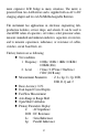
Cs : Serial Capacitance Cp : Parallel Capacitance Second Parameter Display: θ : Phase Angle ESR : Equivalence Serial Resistance D : Dissipation Factor Q : Quality Factor Combinations of Display: Serial Mode : Z –θ, Cs – D, Cs – Q, Cs – ESR, Ls – D, Ls – Q, Ls – ESR Parallel Mode : Cp – D, Cp – Q, Lp – D, Lp – Q 1.2 Impedance Parameters Due to the different testing signals on the impedance measurement instrument, there are DC impedance and AC impedance.
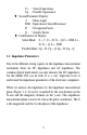
Imaginary Axis Z (Rs , Xs ) Xs Z θ Rs Real Axis Figure 1.1 Z = Rs + jX s = Z ∠θ (Ω ) Rs = Z Cosθ Z = Rs + X s 2 Xs Rs X s = Z Sinθ θ = Tan −1 2 Z = (Impedance) RS = (Resistance ) X S = (Reactance) Ω = (Ohm ) There are two different types of reactance: Inductive (XL) and Capacitive (XC).
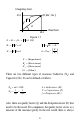
some associated resistance that dissipates power, decreasing the amount of energy that can be recovered. The quality factor can be defined as the ratio of the stored energy (reactance) and the dissipated energy (resistance). Q is generally used for inductors and D for capacitors. 1 1 = D tan δ X s ωL s 1 = = = Rs Rs ωC s R s B = G Rp Rp = = = ωC p R p X p ωL p Q= There are two types of the circuit mode. One is series mode, the other is parallel mode. See Figure 1.
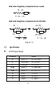
Real and imaginary components are serial Rs jXs Z = Rs + jX s Real and imaginary components are Parallel Rp G=1/Rp jXp jB=1/jXp 1 1 Y= + RP jX P Y = G + jB Figure 1.2 1.3 Specification LCD Display Range: Parameter Z L C DCR ESR D Q θ 0.000 Ω 0.000 µH 0.000 pF 0.000 Ω 0.000 Ω 0.000 0.000 -180.0 ° 6 Range to 9999 MΩ to 9999 H to 9999 F to 9999 MΩ to 9999 Ω to 9999 to 9999 to 180.
Accuracy (Ae): Z Accuracy: |Zx| Freq. DCR 100Hz 120Hz 1KHz 10KHz 100KHz (886) 20M ~ 10M ~ 1M ~ 100K ~ 10 ~ 1 1 ~ 0.1 10M 1M 100K 10 (Ω) (Ω) (Ω) (Ω) (Ω) (Ω) 2% ±1 1% ±1 0.5% ±1 0.2% ±1 0.5% ±1 1% ±1 5% ±1 2% ±1 NA 5%±1 2%±1 0.4% ±1 2%±1 5%±1 Note : 1.The accuracy applies when the test level is set to 1Vrms. 2.Ae multiplies 1.25 when the test level is set to 250mVrms. 3.Ae multiplies 1.50 when the test level is set to 50mVrms. 4.When measuring L and C, multiply Ae by 1+ Dx 2 if the Dx>0.1.
C Accuracy : 100Hz 120Hz 1KHz 10KHz 79.57 pF | 159.1 pF 2% ± 1 66.31 pF | 132.6 pF 2% ± 1 7.957 pF | 15.91 pF 2% ± 1 0.795 pF | 1.591 pF 5% ± 1 NA 100KHz (886) NA 159.1 pF | 1.591 nF 1% ± 1 132.6 pF | 1.326 nF 1% ± 1 15.91 pF | 159.1 pF 1% ± 1 1.591 pF | 15.91 pF 2% ± 1 0.159 pF | 1.591 pF 5% ± 1 1.591 nF | 15.91 nF 0.5% ±1 1.326 nF | 13.26 nF 0.5% ±1 159.1 pF | 1.591 nF 0.5% ±1 15.91 pF | 159.1 pF 0.5% ±1 1.591 pF | 15.91 pF 2%± 1 8 15.91 nF | 159.1 uF 0.2% ±1 13.26 nF | 132.6 uF 0.
L Accuracy : 100Hz 120Hz 1KHz 10KHz 100KHz (886) 31.83 KH | 15.91 KH 2% ± 1 26.52 KH | 13.26 KH 2% ± 1 31.83 KH | 1.591 KH 2% ± 1 318.3 H | 159.1 H 5% ± 1 31.83 H | 15.91 H NA 15.91 KH | 1591 H 1% ± 1 13.26 KH | 1326 H 1% ± 1 1.591 KH | 159.1 H 1% ± 1 159.1 H | 15.91 H 2% ± 1 15.91 H | 1.591 H 5% ± 1 1591 H | 159.1 H 0.5% ±1 1326 H | 132.6 H 0.5% ±1 159.1 H | 15.91 H 0.5% ±1 15.91 H | 1.591 H 0.5% ±1 1.591 H | 159.1 mH 2%± 1 9 159.1 H | 15.91 mH 0.2% ±1 132.6 H | 13.26 mH 0.2% ±1 15.
D Accuracy : |Zx| Freq. 100Hz 20M ~ 10M (Ω) ±0.020 10M ~ 1M (Ω) ±0.010 1M ~ 100K (Ω) ±0.005 100K ~ 10 (Ω) ±0.002 10 ~ 1 1 ~ 0.1 (Ω) ±0.005 (Ω) ±0.010 ±0.050 NA ±0.020 ±0.050 ±0.020 ±0.004 ±0.020 ±0.050 20M ~ 10M (Ω) ±1.046 10M ~ 1M (Ω) ±0.523 1M ~ 100K (Ω) ±0.261 100K ~ 10 (Ω) ±0.105 10 ~ 1 1 ~ 0.1 (Ω) ±0.261 (Ω) ±0.523 ±2.615 NA ±1.046 ±1.046 ±0.209 ±1.046 ±2.615 120Hz 1KHz 10KHz 100KHz (886) θ Accuracy : |Zx| Freq. 100Hz 120Hz 1KHz 10KHz 100KHz (886) ±2.
Z Accuracy: As shown in table 1. C Accuracy: Zx = 1 2 ⋅ π ⋅ f ⋅ Cx CAe = Ae of |Zx| f : Test Frequency (Hz) Cx : Measured Capacitance Value (F) |Zx| : Measured Impedance Value (Ω) Accuracy applies when Dx (measured D value) ≦ 0.1 When Dx > 0.1, multiply CAe by 1 + Dx 2 Example: Test Condition: Frequency : 1KHz Level : 1Vrms Speed : Slow DUT : 100nF Then 1 Zx = 2 ⋅ π ⋅ f ⋅ Cx 1 = = 1590Ω 2 ⋅ π ⋅ 103 ⋅ 100 ⋅ 10 − 9 Refer to the accuracy table, get CAe=±0.
L Accuracy: Zx = 2 ⋅ π ⋅ f ⋅ Lx LAe = Ae of |Zx| f : Test Frequency (Hz) Lx : Measured Inductance Value (H) |Zx| : Measured Impedance Value (Ω) Accuracy applies when Dx (measured D value) ≦ 0.1 When Dx > 0.1, multiply LAe by 1 + Dx 2 Example: Test Condition: Frequency : 1KHz Level : 1Vrms Speed : Slow DUT : 1mH Then Zx = 2 ⋅ π ⋅ f ⋅ Lx = 2 ⋅ π ⋅ 103 ⋅ 10 − 3 = 6.283Ω Refer to the accuracy table, get LAe=±0.
ESRAe = Ae of |Zx| f : Test Frequency (Hz) Xx : Measured Reactance Value (Ω) Lx : Measured Inductance Value (H) Cx : Measured Capacitance Value (F) Accuracy applies when Dx (measured D value) ≦ 0.1 Example: Test Condition: Frequency : 1KHz Level : 1Vrms Speed : Slow DUT : 100nF Then 1 Zx = 2 ⋅ π ⋅ f ⋅ Cx 1 = = 1590Ω 3 2 ⋅ π ⋅ 10 ⋅ 100 ⋅ 10 − 9 Refer to the accuracy table, get CAe=±0.2%, Ae ESR Ae = ± Xx ⋅ = ±3.
DAe = Ae of |Zx| Accuracy applies when Dx (measured D value) ≦ 0.1 When Dx > 0.1, multiply Dx by (1+Dx) Example: Test Condition: Frequency : 1KHz Level : 1Vrms Speed : Slow DUT : 100nF Then 1 Zx = 2 ⋅ π ⋅ f ⋅ Cx 1 = = 1590Ω 3 2 ⋅ π ⋅ 10 ⋅ 100 ⋅ 10 − 9 Refer to the accuracy table, get CAe=±0.2%, Ae D Ae = ± ⋅ = ±0.
Accuracy applies when Qx ⋅ De < 1 Example: Test Condition: Frequency : 1KHz Level : 1Vrms Speed : Slow DUT : 1mH Then Zx = 2 ⋅ π ⋅ f ⋅ Lx = 2 ⋅ π ⋅ 103 ⋅ 10 − 3 = 6.283Ω Refer to the accuracy table, get LAe=±0.5%, Ae De = ± ⋅ = ±0.005 100 If measured Qx = 20 Then Qx 2 ⋅ De Q Ae = ± 1 Qx ⋅ De 2 =± 1 0.
Example: Test Condition: Frequency : 1KHz Level : 1Vrms Speed : Slow DUT : 100nF Then 1 Zx = 2 ⋅ π ⋅ f ⋅ Cx 1 = = 1590Ω 3 2 ⋅ π ⋅ 10 ⋅ 100 ⋅ 10 − 9 Refer to the accuracy table, get ZAe=±0.2%, 180 Ae θ Ae = ± ⋅ π 100 180 0.2 =± ⋅ = ±0.115 deg π 100 Testing Signal: Level Accuracy Frequency Accuracy : ± 5% : 0.1% Output Impedance : 100Ω ± 5% Measuring Speed: Fast : 4.5 meas. / sec. Slow : 2.5 meas. / sec.
General: Temperature : 0°C to 70°C (Operating) -20°C to 70°C (Storage) Relative Humidity : Up to 85% Battery Type : 2 AA size Ni-Mh or Alkaline Battery Charge : Constant current 150mA approximately Battery Operating Time : 2.5 Hours typical AC Operation : 110/220V AC, 60/50Hz with proper adapter Low Power Warning : under 2.2V Dimensions : 174mm x 86mm x 48mm (L x W x H) 6.9” x 3.4” x 1.9” Weight : 470g Considerations Test Frequency. The test frequency is user selectable and can be changed.
Charged Capacitors Always discharge any capacitor prior to making a measurement since a charged capacitor may seriously damage the meter. Effect Of High D on Accuracy A low D (Dissipation Factor) reading is desirable. Electrolytic capacitors inherently have a higher dissipation factor due to their normally high internal leakage characteristics. If the D (Dissipation Factor) is excessive, the capacitance measurement accuracy may be degraded.
Even if the manufacturers’ specification is not known, the capacitance of a measured length of cable (such as 10 feet) can be used to determine the capacitance per foot; do not use too short a length such as one foot, because any error becomes magnified in the total length calculations. Sometimes, the capacitance of switches, interconnect cables, circuit board foils, or other parts, affecting stray capacitance can be critical to circuit design, or must be repeatable from one unit to another.
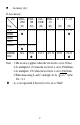
Carrying Case (Optional) 20
2. Operation 2.1 Physical Description 1. 3. 5. 7. 9. 11. 13. 15. 17. 19. G UARD H POT L POT H CUR L CUR G UARD NA Secondary Parameter Display Model Number Relative Key Open/Short Calibration Key Display Update Speed Key Range Hold Key Battery Charge Indicator Guard Terminal LPOT/LCUR Terminal 2. 4. 6. 8. 10. 12. 14. 16. 18. 20.
2.2 Making Measurement 2.2.1 Battery Replacement When the LOW BATTERY INDICATOR lights up during normal operation, the batteries in the Models 885 & 886 should be replaced or recharged to maintain proper operation. Please perform the following steps to change the batteries: 1. Remove the battery hatch by unscrewing the screw of the battery compartment. 2. Take out the old batteries and insert the new batteries into the battery compartment. Please watch out for battery polarity when installing new batteries.
2.2.2 Battery Recharging/AC operation Caution ! Only the Models 885 or 886 standard accessory AC to DC adapter can be used with Model 885. Other battery eliminator or charger may result in damage to Modes 885 or 886. The Models 885 & 886 works on external AC power or internal batteries. To power the Model 885 with AC source, make sure that the Models 885 or 886 is off, then plug one end of the AC to DC adapter into the DC jack on the right side of the instrument and the other end into an AC outlet.
2.2.3 Open and Short Calibration The Models 885 & 886 provides open/short calibration capability so the user can get better accuracy in measuring high and low impedance. We recommend that the user performs open/short calibration if the test level or frequency has been changed. Open Calibration First, remaining the measurement terminals with the open status, then press the CAL key shortly (no more than two second), the LCD will display: This calibration takes about 10 seconds.
2.2.4 Display Speed The Models 885 & 886 provides two different display speeds (Fast/Slow). It is controlled by the Speed key. When the speed is set to fast, the display will update 4.5 readings every second. When the speed is set to slow, it’s only 2.5 readings per second. 2.2.5 Relative Mode The relative mode lets the user to make quick sort of a bunch of components. First, insert the standard value component to get the standard value reading. (Approximately 5 seconds in Fast Mode to get a stable reading.
2.2.7 DC Resistance Measurement The DC resistance measurement measures the resistance of an unknown component by 1VDC. Select the L/C/Z/DCR key to make the DCR measurement. The LCD display: 2.2.8 AC Impedance Measurement The AC impedance measurement measures the Z of an unknown device. Select the L/C/Z/DCR key to make the Z measurement. The LCD display: The testing level and frequency can by selected by pressing the Level key and Frequency key, respectively. 2.2.
shows some examples of capacitance measurement: The testing level and frequency can by selected by pressing the Level key and Frequency key, respectively. 2.2.10 Inductance Measurement Select the L/C/Z/DCR key to Ls or Lp mode for measuring the inductance in serial mode or parallel mode. If the serial mode (Ls) is selected, the D, Q and ESR can be shown on the secondary display. If the parallel mode (Lp) is selected, only the D and Q can be shown on the secondary display.
2.3 Accessory Operation Follow the figures below to attach the test probes for making measurement.
HP LP LC HC TL885B 4-Wire Test Clip TL08C Kelvin Clip 29
4. Application 4.1 Test Leads Connection Auto balancing bridge has four terminals (HCUR, HPOT, LCUR and LPOT) to connect to the device under test (DUT). It is important to understand what connection method will affect the measurement accuracy. 2-Terminal (2T) 2-Terminal is the easiest way to connect the DUT, but it contents many errors which are the inductor and resistor as well as the parasitic capacitor of the test leads (Figure 3.1).
3-Terminal uses coaxial cable to reduce the effect of the parasitic capacitor (Figure 3.2). The shield of the coaxial cable should connect to guard of the instrument to increase the measurement range up to 10MΩ. Ro Lo A HCUR HPOT DUT Co V DUT Co doesn't effect measurement result LPOT LCUR Ro (a) CONNECTION Lo (b) BLOCK DIAGRAM 3T 1m 10m 100m 1 10 100 1K 10K 100K 1M 10M (c) TYPICAL IMPEDANCE MEASUREMENT RANGE(£[) A V DUT (d) 2T CONNECTION WITH SHILDING Figure 3.
resistance (Figure 3.3). This connection can improve the measurement range down to 10mΩ. However, the effect of the test lead inductance can’t be eliminated. A HCUR HPOT DUT V DUT LPOT LCUR (a) CONNECTION (b) BLOCK DIAGRAM 4T 1m 10m 100m 1 10 100 1K 10K 100K 1M 10M (c) TYPICAL IMPEDANCE MEASUREMENT RANGE (£[) Figure 3.3 5-Terminal (5T) 5-Terminal connection is the combination of 3T and 4T (Figure 3.4). It has four coaxial cables.
A HCUR HPOT DUT V DUT LPOT L CUR (a) CONNECTION (b) BLOCK DIAGRAM 5T 1m 10m 100m 1 10 100 1K 10K 100K 1M 10M (c) TYPICAL IMPEDANCE MEASUREMENT RANGE (£[) A V DUT (d) WRONG 4T CONNECTION Figure 3.4 4-Terminal Path (4TP) 4-Terminal Path connection solves the problem that caused by the test lead inductance. 4TP uses four coaxial cables to isolate the current path and the voltage sense cable (Figure 3.5). The return current will flow through the coaxial cable as well as the shield.
measurement range from 1mΩ to 10MΩ. HCUR V HPOT DUT DUT LPOT LCUR A (a) CONNECTION (b) BLOCK DIAGRAM HCUR HPOT 4T DUT LPOT 1m 10m 100m 1 10 100 1K 10K 100K 1M 10M (c) TYPICAL IMPEDANCE MEASUREMENT RANGE(£[) LCUR (d) 4T CONNECTION WITH SHILDING Figure 3.5 Eliminating the Effect of the Parasitic Capacitor When measuring the high impedance component (i.e. low capacitor), the parasitic capacitor becomes an important issue (Figure 3.6). In figure 3.
HCUR HPOT LPOT LCUR Cd HPOT LPOT LCUR Guard Plant DUT Ch HCUR Connection Point Cl Ground (b) Guard Plant reduces Parastic Effect (a) Parastic Effect Figure 3.6 4.2 Open/Short Compensation For those precision impedance measuring instrument, the open and short compensation need to be used to reduce the parasitic effect of the test fixture. The parasitic effect of the test fixture can be treated like the simple passive components in figure 3.7(a).
Parastic of the Test Fixture Redundant (Zs) Impedance HCUR Rs Parastic (Yo) Conductance Ls HPOT Zm Co Zdut Go LPOT LCUR (a) Parastic Effect of the Test Fixture HCUR Rs Ls HPOT Yo Co Go OPEN LPOT LCUR Yo = Go + j£sCo 1 (Rs + j£s<< ) Go+j£sCo (b) OPEN Measurement HCUR Rs Ls HPOT Zs Co LPOT LCUR Zs = Rs + j£sLs (c) SHORT Measurement Figure 3.
Zs Zm Yo Zdut Zdut = Zm - Zs 1-(Zm-Zs)Yo (d) Compensation Equation Figure 3.7 (Continued) 4.3 Selecting the Series or Parallel Mode According to different measuring requirement, there are series and parallel modes to describe the measurement result. It is depending on the high or low impedance value to decide what mode to be used. Capacitor The impedance and capacitance in the capacitor are negatively proportional.
Small capacitor (High impedance) C RP Large capacitor (Low impedance) C RP No Effect Effect RS RS No Effect Effect Figure 3.8 Inductor The impedance and inductive in the inductor are positively proportional. Therefore, the large inductor equals to the high impedance and vice versa. Figure 3.9 shows the equivalent circuit of inductor. If the inductor is small, the Rs is more important than the Rp. If the inductor is large, the Rp should be taking care of.
Large inductor (High impedance) Small inductor (Low impedance) L L RP RP No Effect Effect RS RS No Effect Effect Figure 3.
5. Limited Three-Year Warranty B&K Precision Corp. warrants to the original purchaser that its products and the component parts thereof, will be free from defects in workmanship and materials for a period of three years from date of purchase. B&K Precision Corp. will, without charge, repair or replace, at its option, defective product or component parts. Returned product must be accompanied by proof of the purchase date in the form of a sales receipt. To obtain warranty coverage in the U.S.A.
Service Information Warranty Service: Please return the product in the original packaging with proof of purchase to the below address. Clearly state in writing the performance problem and return any leads, connectors and accessories that you are using with the device. Non-Warranty Service: Return the product in the original packaging to the below address. Clearly state in writing the performance problem and return any leads, connectors and accessories that you are using with the device.
6. Safety Precaution SAFETY CONSIDERATIONS The Models 885 & 886 LCR Meter has been designed and tested according to Class 1A 1B or 2 according to IEC479-1 and IEC 721-3-3, Safety requirement for Electronic Measuring Apparatus. SAFETY PRECAUTIONS SAFETY NOTES The following general safety precautions must be observed during all phases of operation, service, and repair of this instrument.
SAFETY SYMBOLS Caution, risk of electric shock Earth ground symbol Equipment protected throughout by double insulation or reinforced insulation ! Caution (refer to accompanying documents) DO NOT SUBSTITUTE PARTS OR MODIFY INSTRUMENT Because of the danger of introducing additional hazards, do not install substitute parts or perform any unauthorized modification to the instrument. Return the instrument to a qualified dealer for service and repair to ensure that safety features are maintained.
Tabla de Contendido 1. INTRODUCCIÓN ............................................................. 45 GENERAL .......................................................................... 45 PARÁMETROS DE IMPEDANCIA ......................................... 47 ESPECIFICACIÓN ............................................................... 50 ACCESSORIOS ................................................................... 63 2. OPERACIÓN ..................................................................... 64 2.
1. Introducción 1.1 General Los Modelos 885 & 886 de B&K Precision,Medidor LCR/ESR en circuito es un instrumento portátil de alta precisión para medir inductores, capacitores y resistores con una precisión del 0.5%. Es el instrumento portátil más avanzado a la fecha. El 885 u 886 puede ayudar a ingenieros y estudiantes a comprender las componentes y a efectuar servicio de equipos en el taller electrónico. Los rangos del instrumento pueden ser automáticos o manuales.
Estos versátiles modelos pueden realizar virtualmente todas las funciones de puentes LCR. Este económico medidor puede sustituIr a un Puente LCR, con una precisión básica del 0.2%. Opera con dos baterías AA y se entrega con un adaptador cargador AC a DC y dos baterías AA Ni-Mh recargables. El instrumento se emplea en escuelas, laboratorios, líneas de producción y talleres de servicio.
Cp : Capacitancia paralelo Visualización de parámetro secundario: θ : Angulo de fase ESR : Resistencia serial equivalente D : Factor de disipación Q : Factor de calidad Combinaciones de visualización : Modo serial : Z –θ, Cs – D, Cs – Q, Cs – ESR, Ls – D, Ls – Q, Ls – ESR Modo paralelo : Cp – D, Cp – Q, Lp – D, Lp – Q 1.2 Parámetros de impedancia Debido a las diferentes señales de medición, existe la impedancia DC y AC.
Eje imaginario Z (Rs , Xs ) Xs Z θ Rs Eje real Figura 1.1 Z = Rs + jX s = Z ∠θ (Ω ) Rs = Z Cosθ Z = Rs + X s 2 Xs Rs X s = Z Sinθ θ = Tan −1 2 Z = (Impedance) RS = (Resistance) X S = (Reactance) Ω = (Ohm ) Existen dos tipos de reactancia: Inductiva (XL) y Capacitiva (XC). Pueden definirse como sigue X L = ωL = 2πfL 1 = 1 XC = ωC 2πfC L = Inductance (H) C = Capacitance (F) f = Frequency (Hz) Debemos considerar también el factor de calidad (Q) y el factor de disipación (D).
inductores y D para capacitores. 1 1 = D tan δ X s ωL s 1 = = = Rs Rs ωC s R s B = G Rp Rp = = = ωC p R p X p ωL p Q= Modos. Hay dos tipos: Modo serie y modo paralelo. Vea la Figura 2 para relacionarlos.
Los componentes real e imaginario son seriales Rs jXs Z = Rs + jX s Los componentes real e imaginario son paralelos Rp G=1/Rp jXp jB=1/jXp 1 1 Y= + RP jX P Y = G + jB Figura 1.2 1.3 Especificación Rango de pantalla LCD: Parámetro Z L C DCR ESR D Q θ Precisión(Ae): 0.000Ω 0.000µH 0.000pF 0.000Ω 0.000Ω 0.000 0.000 -180.0° Precisión de Z: 50 Rango to 9999MΩ to 9999H to 9999F to 9999MΩ to 9999Ω to 9999 to 9999 to 180.
|Zx| Freq. DCR 100Hz 120Hz 1KHz 10KHz 100KHz (886) 20M ~ 10M (Ω) 2% ±1 10M ~ 1M ~ 100K ~ 10 ~ 1 1 ~ 0.1 1M 100K 10 (Ω) (Ω) (Ω) (Ω) (Ω) 1% ±1 0.5% ±1 0.2% ±1 0.5% ±1 1% ±1 5% ±1 NA 2% ±1 5%±1 2%±1 0.4% ±1 2%±1 5%±1 Note : 1.La precisión aplica con el nivel de prueba de 1Vrms. 2.Multiplicar Ae por 1.25 con nivel de 250mVrms. 3. Multiplicar Ae por 1.5 con nivel de 50mVrms. 4.Al medir L y C, multiplicar Ae por 1+ Dx : Ae no se especifica con el nivel de 50mV. 51 2 si Dx>0.1.
Precisión de C: 100Hz 120Hz 1KHz 10KHz 79.57 pF | 159.1 pF 2% ± 1 66.31 pF | 132.6 pF 2% ± 1 7.957 pF | 15.91 pF 2% ± 1 0.795 pF | 1.591 pF 5% ± 1 NA 100KHz (886) NA 159.1 pF | 1.591 nF 1% ± 1 132.6 pF | 1.326 nF 1% ± 1 15.91 pF | 159.1 pF 1% ± 1 1.591 pF | 15.91 pF 2% ± 1 0.159 pF | 1.591 pF 5% ± 1 1.591 nF | 15.91 nF 0.5% ±1 1.326 nF | 13.26 nF 0.5% ±1 159.1 pF | 1.591 nF 0.5% ±1 15.91 pF | 159.1 pF 0.5% ±1 1.591 pF | 15.91 pF 2%± 1 52 15.91 nF | 159.1 uF 0.2% ±1 13.26 nF | 132.6 uF 0.
Precisión de L: 31.83 KH | 15.91 100Hz KH 2% ± 1 26.52 KH | 13.26 120Hz KH 2% ± 1 31.83 KH | 1.591 1KHz KH 2% ± 1 318.3 H | 159.1 10KHz H 5% ± 1 31.83 H | 100KHz 15.91 (886) H NA 15.91 KH | 1591 H 1% ± 1 13.26 KH | 1326 H 1% ± 1 1.591 KH | 159.1 H 1% ± 1 159.1 H | 15.91 H 2% ± 1 15.91 H | 1.591 H 5% ± 1 1591 H | 159.1 H 0.5% ±1 1326 H | 132.6 H 0.5% ±1 159.1 H | 15.91 H 0.5% ±1 15.91 H | 1.591 H 0.5% ±1 1.591 H | 159.1 mH 2%± 1 53 159.1 H | 15.91 mH 0.2% ±1 132.6 H | 13.26 mH 0.2% ±1 15.
Precisión de D: |Zx| Freq. 100Hz 20M ~ 10M ~ 1M ~ 100K ~ 10 ~ 1 1 ~ 0.1 10M 1M 100K 10 (Ω) (Ω) (Ω) (Ω) (Ω) (Ω) ±0.020 ±0.010 ±0.005 ±0.002 ±0.005 ±0.010 120Hz 1KHz 10KHz 100KHz (886) ±0.050 ±0.020 NA ±0.050 ±0.020 ±0.004 ±0.020 ±0.050 Precisión de θ : |Zx| Freq. 100Hz 20M ~ 10M ~ 1M ~ 100K ~ 10 ~ 1 1 ~ 0.1 10M 1M 100K 10 (Ω) (Ω) (Ω) (Ω) (Ω) (Ω) ±1.046 ±0.523 ±0.261 ±0.105 ±0.261 ±0.523 120Hz 1KHz 10KHz 100KHz (886) ±2.615 ±1.046 NA ±2.615 ±1.046 ±0.209 ±1.046 ±2.
Precisión de Z: Como se muestra en la tabla 1. Precisión de C: Zx = 1 2 ⋅ π ⋅ f ⋅ Cx CAe = Ae de |Zx| f : Frecuencia de prueba (Hz) Cx : Valor medido de capacitancia (F) |Zx| : Valor medido de impedancia (Ω) La precisión aplica cuando Dx (Valor medido D ) ≦ 0.1 Cuando Dx > 0.
Lx : Valor medido de inductancia (H) |Zx| : Valor medido de imperdancia(Ω) La precisión aplica cuando Dx (Valor medido D ) ≦ 0.1 Cuando Dx > 0.1, multiplique CAe por 1 + Dx 2 Ejemplo: Condición de prueba: Frecuencia : 1KHz Nivel : 1Vrms Velocidad : Lenta DUT : 1mH Entonces Zx = 2 ⋅ π ⋅ f ⋅ Lx = 2 ⋅ π ⋅ 103 ⋅ 10 − 3 = 6.283Ω Refiriéndose a la tabla de precisión, obtenemos LAe=±0.
La precisión aplica cuando Dx ≦ 0.1 Ejemplo: Condición de prueba: Frecuencia : 1KHz Nivel : 1Vrms Velocidad : Lenta DUT : 100nF Entonces 1 2 ⋅ π ⋅ f ⋅ Cx 1 = = 1590Ω 3 2 ⋅ π ⋅ 10 ⋅ 100 ⋅ 10 − 9 Zx = Refiriéndose a la tabla, obtenemos CAe=±0.2%, ESR Ae = ± Xx ⋅ Ae = ±3.18Ω 100 Precisión D: D Ae = ± Ae 100 DAe = Ae of |Zx| La precisión aplica cuando Dx (Valor medido D ) ≦ 0.1 Cuando Dx > 0.
1 2 ⋅ π ⋅ f ⋅ Cx 1 = = 1590Ω 3 2 ⋅ π ⋅ 10 ⋅ 100 ⋅ 10 − 9 Zx = Refiriéndose a la tabla de precisión, obtenemos CAe=±0.2%, D Ae = ± ⋅ Ae = ±0.002 100 Precisión de Q: Q Ae =± 2 Qx ⋅ De 1 Qx ⋅ De QAe = Ae de |Zx| Qx : Valor del factor de calidad medido De : Precisión relativa de De La precisión aplica si Qx ⋅ De < 1 Ejemplo: Condición de prueba: Frecuencia : 1KHz Nivel : 1Vrms Velocidad : Lenta DUT : 1mH Entonces Zx = 2 ⋅ π ⋅ f ⋅ Lx = 2 ⋅ π ⋅ 103 ⋅ 10 − 3 = 6.
Refiriéndose a la tabla de precisión, obtenemos LAe=±0.5%, De = ± ⋅ Ae = ±0.005 100 Si Qx = 20 (medido) Entonces Q Ae = ± =± Qx 2 ⋅ De 1 Qx ⋅ De 2 1 0.1 Precisión de θ : θe = 180 Ae ⋅ π 100 Ejemplo: Condición de prueba: Frecuencia: 1KHz Nivel : 1Vrms Velocidad : Lenta DUT : 100nF Entonces 1 2 ⋅ π ⋅ f ⋅ Cx 1 = = 1590Ω 3 2 ⋅ π ⋅ 10 ⋅ 100 ⋅ 10 − 9 Zx = Refiriéndose a la tabla de precisión, obtenemos ZAe=±0.
180 Ae ⋅ π 100 180 0.2 =± ⋅ = ±0.115 deg π 100 θ Ae = ± Señal de prueba: Precisión del nivel : ± 5% Precisión de la frecuencia : 0.1% Impedancia de salida : 100Ω ± 5% Velocidad de medición: Rápida : 4.5 meas. / sec. Lenta : 2.5 meas. / sec. General: Temperatura : 0°C to 70°C (Operativa) -20°C to 70°C (Almacenamiento) Humedad relativa : Hasta 85% Batería : 2 AA Ni-Mh o Alcalina Carga de batería : Corriente constante 150mA aproximada Tiempo de operación : 2.
Consideraciones Frecuencia de prueba. La frecuencia puede seleccionarse y cambiarse. Generalmente se usa una señal de 1KHz o mayor para medir capacitores de 0.01uF o menores y una señal de 120Hz para capacitores 10uF o mayores. Típicamente se usa una señal de prueba de 1KHz o mayor para medir inductores usados en circuitos de audio y RF (radio frecuencia), dado que estos componentes operan a frecuencias mayores y deben medirse arriba de 1KHz.
Medición de la capacitancia de cables, switches u otros componentes La medición de la capacitancia de un cable coaxial es muy importatnte para determinar su longitud. La mayoría de los fabricantes indican la capacitancia por pie, por lo que es posible determinar la longitud del cable midiendo su capacitancia. Ejemplo: Para un cable con una capacitancia de 10pF por pie, obtenemos una lectura de 1.000nF. Dividiendo 1000pF (1.
1.
2. Operación 2.1 Descripción física G UARD H POT L POT H CUR L CUR G UARD 1. 3. 5. 7. 9. NA Pantalla secundaria Núemro de modelo Tecla relativa Tecla de Calibracion corto/abierto 11. Tecla de actualización de velocidad de visualización 13. Tecla de retención de rango 2. Pantalla primaria 4. Indicador de batería baja 6. Switch de encendido 8. Tecla de nivel de medición 10. Tecla de frecuencia de medición 12. Tecla de funciónD/Q/θ/ESR 14.
15. Indicador de dcarga de batería 17. Guard Terminal 19. LPOT/LCUR Terminal 16. Entrada del adaptador DC 18. HPOT/HCUR Terminal 20. Compartimiento de batería 2.2 Efectuando mediciones 2.2.1 Reemplazo de baterías Cuando el LOW BATTERY INDICATOR enciende durante operación normal, las baterías en los Modelos 885 & 886 deben reemplazarse o recargarse para una operación correcta. Para cambiarlas, siga los pasos siguientes: 1. Remueva la compuerta desatornillando el tornillo del compartimiento de la batería.
Battery Replacement 2.2.2 Recarga de batería/operación AC ! Precaución Use solo el adaptador estándar AC a DC en el modelo 885. Otros eliminadores o cargadores pueden dañar a los modelos 885 y 886 Los Modelos 885 & 886 operan con fuente de AC o con baterías internas.
2.2.3 Calibración/corto circuito abierto (open/short) Los Modelos 885 & 886 proveen calibración open/short para que el usuario obtenga mayor precisión al medir baja y alta impedancia. Recomendamos usar la calibración al cambiar la frecuencia o nivel de señal de prueba. : Calibración Open Mantenga las terminales de medición abiertas, y presione luego la tecla CAL brevemente (no más de dos segundos); La pantalla mostrará: Este proceso dura alrededor de 10 segundos.
modelo 885 emitirá un breve sonido (beep).
2.3.1 Velocidad de visualización Los Modelos 885 & 886 proveen dos velocidades en pantalla (Fast/Slow), controladas por la tecla Speed . En la posición fast, la pantalla se actualiza 4.5 lecturas cada segundo. En slow, son sólo 2.5 lecturas por segundo. 2.3.2 Modo relativo El modo relative permite al usuario efectuar un ordenamiento rápido de un lote de components. Inserte primeramente el componente de valor estándar para obtener su valos. (Aproximadamente 5 segundos en Modo rápido para una lectura estable.
La pantalla exhibirá: 2.3.5 Medición de impedancia AC Proceso para medir el valor de impedancia AC Z de un dispositivo de valor desconocido. Seleccione la tecla L/C/Z/DCR . La pantalla exhibirá: El nivel de prueba y la frecuencia se seleccionan con las teclas Level y Frequency respectivamente. 2.3.6 Medición de Capacitancia Para medir la capacitancia de una componente, seleccione la tecla L/C/Z/DCR para los modos Cs (serial) o Cp (paralelo).
El nivel de prueba y la frecuencia se seleccionan con las teclas Level y Frequency respectivamente. 2.3.7 Medición de inductancia Seleccione la tecla L/C/Z/DCR para el modo Ls (serial) o Lp(paralelo) de medición de inductancia. En el modo serial los valores de D, Q y ESR pueden exhibirse en la pantalla secundaria. En el modo paralelo (Lp), sólo se muestran los valores de D y Q en la pantalla secundaria.
2.4 Operación de los accesorios Refiérase a las figures siguientes para la conexión de los accesorios.
HP LP LC HC TL885B Clip de 4 puntas TL08C Kelvin Clip 73
3. Aplicación 3.1 Conexión de las puntas de prueba El Puente autobalanceado tiene 4 puntas (HCUR, HPOT, LCUR y LPOT) para conectarlas al dispositivo bajo prueba (DUT). Es importante entender como el método de conexión afecta la precision de la medición. 2-Terminal (2T) 2-Terminal es la manera más sencilla de conectar el DUT, pero introduce errores debido a la inductancia,resistencia capacitancia parásitas de las puntas (Figura 3.1).
capacitor parásito (Figure 3.2). El blindaje del cable coaxial debe conectarse al común del instrumento para incrementar el rango de medición hasta 10MΩ. Ro Lo A HCUR HPOT DUT Co V DUT Co doesn't effect measurement result LPOT LCUR Ro (a) CONNECTION Lo (b) BLOCK DIAGRAM 3T 1m 10m 100m 1 10 100 1K 10K 100K 1M 10M (c) TYPICAL IMPEDANCE MEASUREMENT RANGE(£[) A V DUT (d) 2T CONNECTION WITH SHILDING Figura 3.
eliminarse el efecto de la inductancia de las puntas de prueba. A HCUR HPOT DUT V DUT LPOT LCUR (a) CONNECTION (b) BLOCK DIAGRAM 4T 1m 10m 100m 1 10 100 1K 10K 100K 1M 10M (c) TYPICAL IMPEDANCE MEASUREMENT RANGE (£[) Figure 3.3 5-Terminal (5T) La conexión 5-Terminal es la combinación de 3T y 4T (Figura 3.4). Tiene 4 cables coaxiales. Debido a las ventajas de 3T y 4T, esta conexión puede incrementar ampliamente el rango de medición de 10mΩ a 10MΩ.
A HCUR HPOT DUT V DUT LPOT L CUR (a) CONNECTION (b) BLOCK DIAGRAM 5T 1m 10m 100m 1 10 100 1K 10K 100K 1M 10M (c) TYPICAL IMPEDANCE MEASUREMENT RANGE (£[) A V DUT (d) WRONG 4T CONNECTION Figure 3.4 4-Terminal Path (4TP) 4-Terminal Path resuelve el problema causado por la inductancia de la punta de prueba. 4TP usa 4 cables coaxiales para la trayectoria de corriente y el cable sensor de voltaje (Figura 3.5). La corriente de retorno fluye tanto por el cable coaxial como por el blindaje.
incrementa el rango de medición de 1mΩ a 10MΩ. HCUR V HPOT DUT DUT LPOT LCUR A (a) CONNECTION (b) BLOCK DIAGRAM HCUR HPOT 4T DUT LPOT 1m 10m 100m 1 10 100 1K 10K 100K 1M 10M (c) TYPICAL IMPEDANCE MEASUREMENT RANGE(£[) LCUR (d) 4T CONNECTION WITH SHILDING Figura 3.5 Eliminando el Efecto del Capacitor parásito Al medir una componente de alta impedancia (i.e. capacitor pequeño), el capacitor parásito afecta la medición (Figura 3.6). En la figura 3.
HCUR HPOT LPOT LCUR Cd HPOT LPOT LCUR Guard Plant DUT Ch HCUR Connection Point Cl Ground (b) Guard Plant reduces Parastic Effect (a) Parastic Effect Figura 3.6 3.2 Compensación en circuito corto y abierto La compensación de circuito corto y abierto debe usarse para reducir el efecto parásito de las puntas de prueba. Este efecto puede tratarse como los componentes pasivos en la figura 3.7(a). Al abrir el DUT, el instrumento tiene la conductancia Yp = Gp + jωCp (Figura 3.7(b)).
Parastic of the Test Fixture Redundant (Zs) Impedance HCUR Parastic (Yo) Conductance Ls Rs HPOT Zm Co Zdut Go LPOT LCUR (a) Parastic Effect of the Test Fixture HCUR Rs Ls HPOT Yo Co Go OPEN LPOT LCUR Yo = Go + j£sCo 1 (Rs + j£s<< ) Go+j£sCo (b) OPEN Measurement HCUR Rs Ls HPOT Zs Co LPOT LCUR Zs = Rs + j£sLs (c) SHORT Measurement Figura 3.
Zs Zm Yo Zdut Zdut = Zm - Zs 1-(Zm-Zs)Yo (d) Compensation Equation Figura 3.7 (Continuación) 3.3 Selección del modo serial o paralelo Los resultados de una medición dependen del modo, serial o paralelo. La decisión del modo a usar depende del valor de la impedancia alta o baja. Capacitor La impedancia y capacitancia son inversamente proporcionales. Por tanto, un capacitor grande implica impedancia baja, y uno pequeño una impedancia alta. La Figura 3.
Small capacitor (High impedance) C Large capacitor (Low impedance) RP C RP No Effect Effect RS RS No Effect Effect Figure 3.8 Inductor La impedancia y la inductancia son directamente proporcionales. Por tanto, un inductor grande posee alta impedancia, y uno pequeño baja impedancia. La Figura 3.9 muestra el circuito equivalente del inductor. Si el inductor es pequeño, Rs es más importante que Rp. Si el inductor is grande, Rp es importante.
Large inductor (High impedance) Small inductor (Low impedance) L L RP RP No Effect Effect RS RS No Effect Effect Figure 3.
5. Precaución sobre seguridad CONSIDERATIONES DE SEGURIDAD Los Modelos 885 & 886 LCR Meter se han diseñado y probado de acuerdo con Class 1A 1B o 2 de acuerdo con IEC479-1 e IEC 721-3-3, “Safety requirement for Electronic Measuring Apparatus”. PRECAUTIONES NOTAS SOBRE SEGURIDAD Las siguientes precauciones deben observarse durante todas las fases de operación, servicio, y reparación de este instrumento.
SIMBOLOS DE SEGURIDAD Precaución, riesgo de choque eléctrico Tierra física Protección completa con aislamiento doble o reforzado ! Precaución (Consulte los documentos anexos) NO SUSTITUYA PARTES O MODIFIQUE EL INSTRUMENTO A fin de no introducir riesgos adicionales,, no instale partes substitutas o ejecute modificación no autorizada al instrumento.
Garantía Limitada de Tres Anos B&K Precision Corp. Autorizaciones al comprador original que su productos y componentes serán libre de defectos por el periodo de tres anos desde el día en que se compro. B&K Precision Corp. sin carga, repararemos o sustituir, a nuestra opción, producto defectivo o componentes. Producto devuelto tiene que ser acompañado con prueba de la fecha del la compra en la forma de un recibo de las ventas. Para obtener cobertura en los EE.UU.
Información de Servicio Servicio de Garantía: Por favor regrese el producto en el empaquetado original con prueba de la fecha de la compra a la dirección debajo. Indique claramente el problema en escritura, incluya todos los accesorios que se estan usado con el equipo. Servicio de No Garantía: Por favor regrese el producto en el empaquetado original con prueba de la fecha de la compra a la dirección debajo.
22820 Savi Ranch Parkway Yorba Linda, CA 92887 www.bkprecision.com © 2009 B&K Precision Corp.