ECE 2080 ELECTRICAL ENGINEERING LABORATORY I by A. L. Duke Dan McAuliff CLEMSON UNIVERSITY Revised January 1998 by Michael Hannan Revision 1.
Revision Notes 1991 1998 2008 2010 Authors: A. L. Duke and Dan McAuliff. Original release. Author: Michael Hannan. Reorganization, mostly with same information. Author: James Harriss. General reorganization, corrections, and update. Clarified instructions to reduce equipment damage and blown fuses. Redrew many figures. Rewrote laboratory sessions on SPICE and Oscilloscope. Added equipment list and references. Created common Appendix (A to E) for ECE 2080 and ECE 212.
Table of Contents Revision Notes........................................................................................................................... ii Table of Contents...................................................................................................................... iii Equipment..................................................................................................................................iv References ............................................................
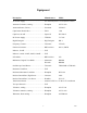
Equipment Description Manufacturer Model AC Power Supply............................................use Autotransformer or Transformer Board Ammeter-Voltmeter, Analog ...........................Hampden ACVA-100 Autotransformer (Variac) ................................Powerstat 3PN116C Capacitance Decade Box .................................EICO 1180 Capacitor, 40 mfd............................................Square D PFC2001C DC Power Supply............................................
References 1. Giorgio Rizzoni, Principles and Applications of Electrical Engineering, Fifth Edition, McGraw-Hill, December 2005. 2. Giorgio Rizzoni, Principles and Applications of Electrical Engineering, Revised Fourth Edition, McGraw-Hill, July 2003. 3. Mahmood Nahvi, Joseph A. Edminister, Schaum's Outline of Electric Circuits, Fourth Edition, December 2002. 4. James W. Nilsson and Susan Riedel, Electric Circuits, 8th Edition, Prentice Hall, May 2007. 5. James W.
Preface This laboratory manual is composed of three parts. Part One provides information regarding the course requirements, recording the experimental data, and reporting the results. Part Two includes the laboratory experiments and problem exercises to be performed.
Introduction This laboratory course operates in co-ordination with the companion lecture course, ECE 2070, Basic Electrical Engineering. Each course complements the other: Several ECE 2080 exercises require knowledge of theory developed in ECE2070, and several assist in understanding ECE 2070 concepts. Preliminary laboratory preparation (“Pre-Lab”) is assigned for most periods. A student who understands this preliminary preparation should be able to complete the exercises during the time scheduled.
Preparing the Laboratory Notebook Laboratory-oriented engineering work, particularly research work, provides information that is usually quite detailed. Records of this work and the results specified are kept in laboratory notebooks. Laboratory notebooks must be complete and clear, since data recorded may provide a basis for calculations, conclusions, recommendations, engineering designs, patents, etc.
Graphs and charts are frequently used during laboratory work to determine validity of the data and to detect immediately anomalies, trends, and unexpected changes in the data; this may avoid a need for repeating the experiment later. It is much more expensive in time and material to set up the experiment a second time needlessly, rather than correcting the problem during the first run. Photographs, charts, oscillograms, diagrams, and other loose sheets are sometimes desirable in a notebook.
Reports General The final result of almost all engineering work includes some sort of report. The information for the report usually comes from the engineer’s notebook, status reports, design information, and other reports. It follows that a good engineer must be skilled at transmitting technical information, whether by a long formal report or by a short telephone conversation. Examples of the types of informational reports commonly used by engineers are: - Routine periodic (e.g.
Judgment must be used in establishing sections and subsections in all types of reports. It is just as inappropriate to have a one page report with twenty section headings as it is to have a fifty-page report with only one heading. Where appropriate, elements may be combined and renamed. In this course, two types of reports will be used: the Laboratory Report and the Memo Report. Both are described in the following paragraphs. Memo Report This should be a brief report limited to a single subject.
should include the report title and the report number. Reports without numbers and names are likely to be misfiled and lost. On a student report, the date should be the date the report is due. Objectives. This section should carefully state the objectives or purpose of the test or experiment. It should be edited very carefully to avoid vagueness and ambiguities.
Laboratory 1: Course Description and Introduction Laboratory #1: Course Description and Introduction Objectives: 1. The establishment of course procedures and policies. 2. The review of basic electricity Policies: Course policies on grading and coursework ethics are determined and made known by the instructor of each section. This course will operate as a problem workshop intermingled among laboratory experiments.
Laboratory 2: Measurement of DC Voltage and Current Laboratory #2: Measurement of DC Voltage and Current Objectives: This exercise introduces the digital multimeter as an instrument for measuring DC voltage, current, and resistance. Pre-Lab Preparation: 1. Read Appendix A: Safety. 2. Read Appendix B: Equipment and Instrument Circuits through Digital Multimeters.
Laboratory 2: Measurement of DC Voltage and Current Equipment Needed: DC Power supply Digital multimeter Resistance decade boxes (2) Procedure: 1. Series Circuit E = 10 V R1 = 33kΩ R2 = 100kΩ a) With the values of R1 and R2 provided, connect the circuit shown above. Use the digital multimeter to measure E, V1, V2, and I. b) Check the relationships: E = V1 +V2 I= E R 1 R2 2. Parallel Circuit E = 10 V R1 = 33kΩ R2 = 100kΩ a) With the values of R1 and R2 provided, connect the circuit shown.
Laboratory 3: Computer Analysis Laboratory #3: Computer Analysis Objectives: This exercise is intended to provide familiarity with computer analysis of electrical circuits. It focuses on interpretation of results obtained from a commercial circuit analysis program. Introduction: The analysis of electronic circuits can be expensive in both time and money, especially as circuitry becomes complicated with many and varied components.
Laboratory 3: Computer Analysis We shall use the simple circuit drawn below as an example. 1000 Ω R1 + – R2 5V 2000 Ω I Figure 3.1: Circuit #1 1. Using the rules for adding series resistances, Kirchhoff’s laws, and Ohm’s law, analyze the circuit of Figure 3.1. Calculate the current I and the voltage drops across each of the resistors. 2. SPICE programs tend to use Node Analysis to analyze circuits. One node labeled ‘0’ serves as the reference (ground) node.
Laboratory 3: Computer Analysis 4. Notice that, except for meters, the circuit of Figure 3.1 is electrically identical to the circuit in the B2 SPICE Analog Tutorial #1, which you did in the Pre-Lab assignment. Vmeter V1 R1 R2 5V 1K 2K Figure 3.3: Schematic from B2 SPICE Analog Tutorial #1 5. Create a table showing the three sets of values for currents and node voltages: (a) your calculation from Ohm’s law and Kirchhoff’s laws; (b) your measured values; and (c) the prediction from B2 SPICE.
Laboratory 3: Computer Analysis 7. Analyze another circuit by hand and again with B2 SPICE: 3Ω + – 60 V 1Ω 6Ω 10 Ω 2Ω 4Ω Figure 3.4: Circuit #2 a) b) c) d) e) Label the nodes in the above circuit. By hand, calculate all of the node voltages and branch currents for the circuit. Create the circuit in B2 SPICE. Use B2 SPICE to simulate the circuit. Save the output. Record the node voltages and branch currents predicted by B2 SPICE.
Laboratory 4: Instrument Characteristics Laboratory #4: Instrument Characteristics Objectives: Understand the effect of introducing a measuring device into a circuit, and how the instrument affects the measurement. Introduction: One well known understanding from quantum mechanics is that the act of looking at (e.g., measuring) any system changes the system’s behavior. That is certainly true for electrical and electronic systems.
Laboratory 4: Instrument Characteristics resistance box in the circuit as shown. Adjust the resistance until the meter reads half of its original value. The internal resistance of the ammeter is now equal to the value of the resistance box. Measure and record this value of RS. RM = RS when the Inew = ½ Iold Theoretical Question: (DO NOT TEST THIS EXPERIMENTALLY!) If RS were removed and if the 10 kΩ resistor were replaced by zero ohms (0 Ω), what would be the current I? 2.
Laboratory 4: Instrument Characteristics h) Set the resistance box to 500 Ω. i) Turn the power supply’s “OUTPUT” ON, without disturbing its voltage setting. j) Record the value of current indicated on the ammeter. k) Turn the power supply’s “OUTPUT” OFF. l) Set the resistance box to 75 Ω. m) Turn the power supply’s “OUTPUT” ON. n) Record the value of current indicated on the ammeter. o) Turn the power supply’s “OUTPUT” OFF.
Laboratory 4: Instrument Characteristics VR I RS and VM I RM . So I VR VM RS RM and RM VM RS VR or RM VM RS V0 VM (4.1) Thus, in the circuit shown below, if, for example, VM is 90% of V0, then RM = 9∙RS. For accuracy, RS should be as close to the value of RM as possible, but in practice any reasonably large RS that allows accurate measurements of V0, VM, and RS can yield reasonably accurate measurement of RM.
Laboratory 4: Instrument Characteristics k) Calculate VR. l) Calculate RM, the internal resistance of the voltmeter. 2. Determine the effect of the voltmeter’s internal resistance on the measurement of voltages. WARNING: Be sure resistors are set as required before applying power to the circuit. For this step of the experiment, do not adjust the voltmeter’s scale or the power supply’s voltage adjustment at any time once measurements have begun. a) Set Digital Multimeter to VOLTS and its scale to 20V.
Laboratory 5: Oscilloscope Laboratory #5: Oscilloscope Objectives: This laboratory exercise introduces the operation and use of the oscilloscope. Introduction: The oscilloscope is an instrument for the analysis of electrical circuits by observing voltage and current waves. It may be used to study wave shape, frequency, phase angle, and time, and to compare the relation between two variables directly on the display screen.
Laboratory 5: Oscilloscope a) Measure VR with the oscilloscope for the following values of R: 10kΩ, 100kΩ, and 1MΩ. b) Calculate the theoretical VR with RSCOPE = infinity (ideal). c) Compare the measured to the calculated results. d) Calculate the oscilloscope’s DC input resistance. Discuss RSCOPE vs. accuracy of VR measured on the oscilloscope. The next steps use the autotransformer (Variac®) as an AC power supply.
Laboratory 5: Oscilloscope 120 mH 100 Ω 10 Vrms a) Estimate the worst-case RMS current that might pass through the resistor and the power dissipated in the resistor by assuming the coil is replaced by a shorting wire. The lowpower resistor decade box has a ½-amp fuse, and the resistors are rated for ½ Watt. Are such ratings adequate for this circuit? If not, be sure to use the Power Resistor decade box for this circuit. b) The 60 Hz AC voltage is approximately 10 Vrms.
Laboratory 6: Problems: Circuit Analysis Methods Laboratory #6: Problems: Circuit Analysis Methods Objectives: 1. Review of mesh and nodal analysis. 2. Review of Thévenin’s Theorem. 3. Review of the principle of superposition. Pre-Lab Preparation: Study the following topics in your textbook, Principles and Applications of Electrical Engineering by Giorgio Rizzoni: Study nodal analysis with current sources and with voltage sources. Study mesh analysis.
Laboratory 6: Problems: Circuit Analysis Methods Superposition Principle (from Rizzoni’s text): In a linear circuit containing N sources, each branch voltage and current is the sum of N voltages and currents, each of which may be computed by setting all but one source equal to zero and solving the circuit containing that single source.
Laboratory 6: Problems: Circuit Analysis Methods 2. For the circuit below, find the Thévenin equivalent circuit as seen from terminals A-B. 3. Use the principle of superposition to calculate the voltages across all of the resistors in the circuit below. In Lab: Work the following problems. 1. Write the mesh equations and determine I in the circuit below.
Laboratory 6: Problems: Circuit Analysis Methods 2. Apply nodal analysis to the following circuit to determine the voltage V. 3. For the following circuit below, find the Thévenin equivalent circuit as seen at A-B. 4. Use superposition to find V below.
Laboratory 7: Network Theorems Laboratory #7: Network Theorems Objectives: The purpose of this assignment is to study certain important network theorems, which are used frequently in circuit analysis, and to improve skills in applying these to practical circuits. Experimental and analytical methods are compared. Pre-Lab Preparation: 1. Review Thévenin’s Theorems for DC circuits and for AC circuits. 2. Review the Superposition Theorem. Safety Precautions: 1.
Laboratory 7: Network Theorems nal contacts on the switches get dirty and give high resistance. If that happens, flip the switch a dozen times or so to clean the contacts and measure again.] b) Set the ammeter scale to its maximum. With the power output off, connect the ammeter from A to B. Turn on the power and measure the short-circuit current, ISC, from A to B, decreasing the meter’s scale setting to produce the most accurate reading. You are using the ammeter’s very low resistance to short A to B.
Laboratory 7: Network Theorems c) Remove the 8V power supply from the original circuit, such that the new circuit becomes the following, and then measure VR. 2.0kΩ 4.7kΩ + VR – 3.3kΩ + 5V – d) Remove the 5V power supply from the original circuit such that the new circuit becomes the following, and then measure VR. 2.0kΩ 8V + – 3.3kΩ 4.7kΩ + VR – e) Verify that the principle of superposition holds: VR = VR (b) + VR (c). Compare the result to your theoretical calculation.
Laboratory 8: Problems: Phasors Laboratory #8: Problems: Phasors Objectives: Analyze steady-state AC circuits. Become familiar with phasors and phasor notation. In Lab: Work the following problems. 1. Convert the following: a) Frequency f = 8 kHz to angular frequency ω. b) Angular frequency ω = 0.5 krad/sec to frequency f. c) Polar form 10-45° to rectangular form. d) Rectangular form 3 + j2 to polar form. e) Sinusoidal function v(t) = 12 cos(377t) to a phasor. f) Phasor 1510° to a sinusoidal function.
Laboratory 8: Problems: Phasors 3. In the circuit below, the current i(t) = 2 cos(377t) A. a) Find the impedance Zab. b) Find the voltage Vab. c) Draw a phasor diagram showing the current and the voltage across each element and the Vab). 4. In the circuit below, the voltage Vcd(t) = 25 cos(377t + 45°) V. a) Find the admittance of the circuit. b) Draw a phasor diagram showing the current in each element, the voltage Vcd, and the phasor current I corresponding to i(t).
Laboratory 9: Problems: AC Power Calculations Laboratory #9: Problems: AC Power Calculations Objectives: Review power in AC circuits, including power factors. In Lab: Work the following problems 1. What is the real power with a current and voltage as follows: I(t) = 2 cos(ωt + π/6) A V(t) = 8 cos(ωt) V 2. An unknown impedance Z is connected across a 380 V, 60 Hz source. This causes a current of 5A to flow and 1500 W is consumed. Determine the following: a. Real Power (kW) b. Reactive Power (kvar) c.
Laboratory 10: AC Measurements Laboratory #10: AC Measurements Objectives: This exercise introduces the operation and use of the AC wattmeter, as well as single-phase series circuits containing resistance, inductance, and capacitance. It uses the oscilloscope to measure the phase shift of current through reactive circuits. Pre-Lab: Study Appendix B regarding Wattmeter, especially “Three-Phase Power Measurements”. Study Appendix D information regarding using the oscilloscope to measure phase shift.
Laboratory 10: AC Measurements Procedure: Connect the following AC circuit. 12 Vrms Change the load ZL, as follows: 1. A resistor of R = 25Ω 2. An inductor of L = 120 mH 3. A capacitor of C = 40 µF 4. R and L in series 5. R and C in series 6. R, L, and C in series Measurements For each of the loads listed above: a) Measure the wattmeter reading. b) Measure the total current. c) Measure the voltage drop across each element. For loads 4-6 also measure the current phase shift.
Laboratory 11: Problems: Operational Amplifiers and Digital Logic Laboratory #11: Problems: Operational Amplifiers and Digital Logic Objectives: 1. Better understanding of networks of analog and digital devices. 2. Familiarity with amplification and digital operation of some interface devices for microprocessors. In Lab: Work the following problems. 1. For the following operational amplifier circuit, a) Find Vout in terms of RI, RF, and Vin. b) Given RI = 10Ω, RF = 20kΩ, and Vin = 3V, what is Vout? 2.
Laboratory 12: Digital Logic Circuits Laboratory #12: Digital Logic Circuits Objectives: To obtain experience with digital circuits. Implementation of BCD to seven segment decoder. Equipment Needed: 7447 BCD to seven segment decoder. Digi-trainer designer board. One 330 ohm resistor chip or seven 330 ohm resistors. Seven segment display. Procedure: 1. DECODER: Connect the inputs of the decoder to the four data switches on the trainer. Use the A input of the decoder as the least significant bit.
Appendix A: Safety Appendix A Safety Electricity, when improperly used, is very dangerous to people and to equipment.
Appendix A: Safety Other injuries may be indirectly caused by electrical accidents, such as burns from exploding oilimmersed switchgear or transformers. Although electric shock is normally associated with contact with high-voltage alternating current (AC), under some circumstances death can occur from voltages substantially less than the nominal 120 volts AC found in residential systems. Electric shock is caused by an electric current passing through a part of the body.
Appendix A: Safety dential, commercial, and industrial systems, such as lighting and heating, are always grounded for greater safety. Communication and computer systems, as well as general electronic equipment (e.g., DC power supplies, oscilloscopes, oscillators, and digital multimeters) are grounded for safety and to prevent or reduce electrical noise, crosstalk, and static.
Appendix A: Safety f) Do not exceed the voltage or current ratings of circuit elements or instruments. This particularly applies to wattmeters, since the current or voltage rating may be exceeded with the needle still reading on the scale. g) Be sure any fuses and circuit breakers are of suitable value. When connecting electrical elements to make up a network in the laboratory, it easy to lose track of various points in the network and accidentally connect a wire to the wrong place.
Appendix A: Safety Treating victims for electrical shock includes four basic steps, shown below, that should be taken immediately. Step two requires qualification in CPR and step three requires knowledge of mouth-to-mouth resuscitation. Everyone who works around voltages that can cause dangerous electrical shock should take advantage of the many opportunities available to become qualified in CPR and artificial respiration. Immediate Steps After Electric Shock 1.
Appendix B: Equipment and Instrument Circuits Appendix B Equipment and Instrument Circuits Electrical engineers measure and use a wide variety of electrical circuit variables, such as voltage, current, frequency, power, and energy, as well as electrical circuit parameters, such as resistance, capacitance, and inductance.
Appendix B: Equipment and Instrument Circuits wire is colored white. The load is contained in a metal case. Now, consider what could happen if the ungrounded black wire came loose and made contact with the metal case. It then becomes possible that a person in contact with the ground, by contact with a metal pipe or wet concrete floor, could complete an electrical circuit, being electrocuted in the process.
Appendix B: Equipment and Instrument Circuits Oscilloscope Grounding Errors The purpose of the ISOLATED supply on your workbench is to enable you to ground points in your test circuits in order to make measurements without drawing a large current through the ground connection and tripping a circuit breaker or “zapping” an instrument. Note that for personal safety, the oscilloscope (“scope”) should be plugged into a NON-ISOLATED outlet. Consider now the scenario shown in Figure B.
Appendix B: Equipment and Instrument Circuits Figure B.7 illustrates another thing you will need to watch out for when taking measurements using a scope. Both Channel 1 and Channel 2 on the scope have ground leads, and those leads are physically connected together at the scope itself. What would happen if you tried to measure both resistor voltages using the set-up shown here? The grounds on Channel 1 and Channel 2 are at the same potential and so would short the 200 Ω resistor.
Appendix B: Equipment and Instrument Circuits One might be tempted to “float” the oscilloscope instead of the circuit being tested. This could be accomplished by removing the ground prong on the scope’s power plug. However, doing this would create a safety hazard, since the oscilloscope’s case would be at the same potential as whatever is connected to the scope probe’s ground. It would then be possible for an individual simultaneously touching the scope and an earth connection to be electrocuted.
Appendix B: Equipment and Instrument Circuits Figure B.4: Equivalent circuit for isolated 120 V, 60 Hz supply with the output voltage level controlled by an autotransformer. Function Generator A function generator is an electronic device that is capable of producing time varying voltages of sinusoidal, rectangular (“square”), or triangular shaped waveforms over a broad frequency range (1 Hz - 5 MHz).
Appendix B: Equipment and Instrument Circuits In the d’Arsonval galvanometer, current through a coil of fine wire develops a magnetic field that opposes the field of a permanent magnet, and so rotates a needle across a scale that is marked off in units of the measured variable. This type of movement is used extensively in DC analog instruments.
Appendix B: Equipment and Instrument Circuits to measure voltage or current. When measuring voltage, the input resistance is relatively large (10 MΩ for DC, 10 MΩ in parallel with 100pF for AC). For current measurements, the input resistance is small (1 Ω for 0.2 A DC; 0.1 Ω for 2.0 A DC). Figure B.11 (b) shows an equivalent circuit for the DMM in the resistance measuring mode. The test current, Itest, varies with the resistance range. (a) (b) Figure B.
Appendix B: Equipment and Instrument Circuits The LCR meter has many other useful features, which are described in the manual. If CAL is displayed in the center area, check the secondary display to see if OPn or Srt is displayed. These indicate that the leads should be either opened or shorted followed by pressing the CAL key, for an automatic calibration.
Appendix B: Equipment and Instrument Circuits Digital Storage Oscilloscope The digital storage oscilloscope (DSO) is now the preferred type of oscilloscope for most industrial applications, although analog oscilloscopes are still widely used. The DSO uses digital memory to store data as long as required without degradation. The digital storage allows bringing into play the enormous array of sophisticated digital signal processing tools for the analysis of complex waveforms in today’s circuitry.
Appendix B: Equipment and Instrument Circuits tors marked with a black dot on the Hampden ACWM-100 wattmeter (Figure B.14). In the wattmeter circuit diagrams in this lab, this connection is labeled “+”. AMPS VOLTS + Jumper Figure B.14: Jumper on wattmeter “+” connection To measure power on a three-phase system one could employ what is called the two wattmeter method, in which two wattmeters are connected as shown in Figure B.15.
Appendix B: Equipment and Instrument Circuits The next step is to relate line currents to phase current I a I ab I ac I c I ca I cb Substituting in for the currents * W1 Re Vab I ab Re Vab Iac* W2 Re Vcb I ca* Re Vcb I cb* Summing the wattmeter readings results in * W1 W2 Re Vab I ab Re Vab I ac* Re Vcb I ca* Re Vcb I cb* Since I ac* I ca* then * W1 W2 Re Vab I ab Re Vab Vcb I ac* Re Vcb I cb* Finally, noting that Vab Vcb V
Appendix B: Equipment and Instrument Circuits Then W1 Vab I a cos 208 36.0 cos 0 66.9 2938 Watts W2 Vcb I c cos 208 36.0 cos 120 180 53.1 7434 Watts P3 W1 W2 2938 7434 10,372 Watts References for Appendix B B-1. J. W. Nilsson and S.A. Riedel, Electric Circuits, Seventh Edition, Upper Saddle River, NJ; Pearson Prentice Hall, 2005. B-2. H. H. Chiang, Electrical and Electronic Instrumentation, New York, NY: John Wiley and Sons. 1984. B-3.
Appendix C: Data Plots Appendix C Data Plots It is often desirable to make a two-dimensional plot of data in order to examine relationships between variables, for example: voltage versus time, current versus time, output voltage versus input voltage, output voltage versus frequency, etc.
Appendix C: Data Plots straight line that you have used a ruler to mark off in linear increments to make your own plotting paper. Figure C.1 Relationship of linear and logarithmic scales. This procedure enables you to construct a set of scales to put your data points on for a quick assessment of the relationship, particularly if you want to compare a linear-linear to a semi-log to a log-log plot to see which gives the best presentation.
Appendix D: Operating Instructions for a Typical Oscilloscope Appendix D Operating Instructions for a Typical Oscilloscope The oscilloscope is an instrument for the analysis of electrical circuits by observation of voltage and current waves. It may be used to study frequency, phase angle, and time, and to compare the relation between two variables directly on the display screen. Perhaps the greatest advantage of the oscilloscope is its ability to display the periodic waveforms being studied.
Appendix D: Operating Instructions for a Typical Oscilloscope If several voltage waveforms are to be studied and must maintain their relative phase positions, the sweep generator must be synchronized to the same voltage during the entire test. In this case, one voltage is applied to the oscilloscope as an external trigger. An independent voltage may be applied to the horizontal input in place of the sweep oscillator voltage. In this case, two independent input voltages are displayed against one another.
Appendix D: Operating Instructions for a Typical Oscilloscope ground to the common ground of the circuit. Exercise great care when making measurements with both terminals above ground potential, as there may be a difference in potential between two instrument cases, causing ground loop currents, faulty readings, and damaged equipment.
Appendix D: Operating Instructions for a Typical Oscilloscope Phase Angle Measurement The difference in phase angle between two waveforms may be measured directly on the oscilloscope with little difficulty. For an oscilloscope with only one vertical input: One wave is chosen as the reverence and applied to the vertical input terminals. This same wave is applied to the external trigger input of the scope.
Appendix D: Operating Instructions for a Typical Oscilloscope Phase and Frequency Measurement by Lissajous Patterns The oscilloscope may be used to compare simultaneously two separate waveforms. When two voltages of the same frequency are impressed on the oscilloscope, one on the vertical and one on the horizontal plates, a straight line results on the screen if the voltages are in phase or 180° out of phase. An ellipse is obtained for other phase angles.
Appendix D: Operating Instructions for a Typical Oscilloscope Y frequency : X frequency Be warned that many presentations of Lissajous patterns report (X frequency) : (Y frequency), which would be the inverse of the ratios shown here. To measure frequency by Lissajous patterns, the unknown signal is applied to the vertical input terminals. Then, a variable signal of known frequency is applied to the horizontal input. The HORIZONTAL DISPLAY must be on external sensitivity.
Appendix E: Tektronix TDS 1002B Oscilloscope Appendix E Tektronix TDS 1002B Oscilloscope Introduction Digital multimeters (DMMs) are extremely useful devices to measure and characterize electrical parameters; however, they have a number of limitations. Whether in ammeter or voltmeter mode, they give a one-number summary of the electricity. Their AC frequency range is limited to audio frequencies: 20 Hz to 20 kHz.
Appendix E: Tektronix TDS 1002B Oscilloscope Tektronix TDS 1002B Oscilloscope Figure E.2: Overview of Tektronix TDS 1002B. The Tektronix TDS 1002B is a two-channel digital storage oscilloscope. Pushing a button in the Menu Select region displays a corresponding menu on the screen adjacent to the option buttons, with the Multipurpose Knob allowing adjustment of continuous variables.
Appendix E: Tektronix TDS 1002B Oscilloscope Vertical Sections To the right of the option buttons are knobs and buttons that control the vertical portions of the graph (see Figure E.3). Typically the display shows a graph of voltage (vertical) vs. time (horizontal). This scope has two channels, so the vertical section is divided into two sub-sections with identical controls for each input. The inputs are called Channel 1 (CH 1) and Channel 2 (CH 2).
Appendix E: Tektronix TDS 1002B Oscilloscope BW Limit (Bandwidth Limit) This menu option sets the bandwidth limit of a channel at either the bandwidth of the oscilloscope (60 MHz) or 20 MHz. A lower bandwidth limit decreases the displayed noise, yielding a clearer display, and also limits the display of higher speed details on the selected signal. Volts/Div This menu option selects the incremental sequence of the VOLTS/DIV knob as Coarse or Fine. The Coarse option defines a 1-2-5 incremental sequence.
Appendix E: Tektronix TDS 1002B Oscilloscope unfiltered. One also specifies the type of signal detail to trigger on, selecting from 11 types of measurements. The MEASURE menu allows waveform measurements to be continuously updated and displayed. There are 11 types of available measurements, from which you can display up to five measurements at a time, one assigned to each Option Button.
Appendix E: Tektronix TDS 1002B Oscilloscope Figure E.8: Typical display. Note: MEASURE display; CH 1 V/div; horizontal time per div; trigger information; trigger point “Trig’d”. The ACQUIRE menu function controls the signal acquisition and processing system, allowing different types of acquisition modes for a signal. ACQUIRE Menu The SAVE/RECALL menu function allows one to save and recall up to 10 oscilloscope setups and 2 waveforms.