E fx-9860G SD fx-9860G User’s Guide http://edu.casio.
GUIDELINES LAID DOWN BY FCC RULES FOR USE OF THE UNIT IN THE U.S.A. (not applicable to other areas). NOTICE This equipment has been tested and found to comply with the limits for a Class B digital device, pursuant to Part 15 of the FCC Rules. These limits are designed to provide reasonable protection against harmful interference in a residential installation.
BEFORE USING THE CALCULATOR FOR THE FIRST TIME... This calculator does not contain any main batteries when you purchase it. Be sure to perform the following procedure to load batteries, reset the calculator, and adjust the contrast before trying to use the calculator for the first time. 1. Making sure that you do not accidently press the o key, slide the case onto the calculator and then turn the calculator over. Remove the back cover from the calculator by pulling with your finger at the point marked 1.
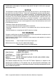
• If the Main Menu shown to the right is not on the display, open the back cover and press the P button located inside of the battery compartment. P button 5. Use the cursor keys (f, c, d, e) to select the SYSTEM icon and press ) to display the contrast adjustment screen. w, then press 1( 6. Adjust the contrast. • The e cursor key makes display contrast darker. • The d cursor key makes display contrast lighter. • 1(INIT) returns display contrast to its initial default. 7.
Quick-Start TURNING POWER ON AND OFF USING MODES BASIC CALCULATIONS REPLAY FEATURE FRACTION CALCULATIONS EXPONENTS GRAPH FUNCTIONS DUAL GRAPH DYNAMIC GRAPH TABLE FUNCTION 20050401
1 Quick-Start Quick-Start Welcome to the world of graphing calculators. Quick-Start is not a complete tutorial, but it takes you through many of the most common functions, from turning the power on, and on to graphing complex equations. When you’re done, you’ll have mastered the basic operation of this calculator and will be ready to proceed with the rest of this user’s guide to learn the entire spectrum of functions available.
2 Quick-Start defc to highlight RUN and then press w. 2. Use • MAT This is the initial screen of the RUN • MAT mode, where you can perform manual calculations, matrix calculations, and run programs. BASIC CALCULATIONS With manual calculations, you input formulas from left to right, just as they are written on paper. With formulas that include mixed arithmetic operators and parentheses, the calculator automatically applies true algebraic logic to calculate the result. Example: 15 × 3 + 61 1.
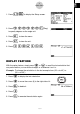
3 Quick-Start SET UP !m to display the Setup screen. 1. Press 2. Press cccccc1(Deg) to specify degrees as the angle unit. 3. Press J to clear the menu. 4. Press o to clear the unit. 5. Press cf*sefw. REPLAY FEATURE d e With the replay feature, simply press or to recall the last calculation that was performed so you can make changes or re-execute it as it is. Example: To change the calculation in the last example from (25 × sin 45˚) to (25 × sin 55˚) 1.
4 Quick-Start FRACTION CALCULATIONS $ You can use the key to input fractions into calculations. The symbol “ { ” is used to separate the various parts of a fraction. Example: 1. Press 2. Press 31/ 16 + 37/9 o. db$bg+ dh$jw. Indicates 871/144 Converting an Improper Fraction to a Mixed Fraction < While an improper fraction is shown on the display, press mixed fraction. !Mto convert it to a < Press !M again to convert back to an improper fraction.
5 Quick-Start EXPONENTS Example: 1250 × 2.065 1. Press o. 2. Press bcfa*c.ag. 3. Press M and the ^ indicator appears on the display. 4. Press f. The ^5 on the display indicates that 5 is an exponent. 5. Press w.
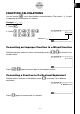
6 Quick-Start GRAPH FUNCTIONS The graphing capabilities of this calculator makes it possible to draw complex graphs using either rectangular coordinates (horizontal axis: x ; vertical axis: y) or polar coordinates (angle: θ ; distance from origin: r). All of the following graphing examples are performed starting from the calculator setup in effect immediately following a reset operation. Example 1: To graph Y = X(X + 1)(X – 2) 1. Press m. defc to highlight GRAPH, and then press w. 2. Use 3.
7 Quick-Start 1(ROOT). Press e for other roots. 2. Press Example 3: Determine the area bounded by the origin and the X = –1 root obtained for Y = X(X + 1)(X – 2) 1. Press !5(G-SLV)6(g). 2. Press 3(∫dx). d to move the pointer to the location where X = –1, and then press w. Next, use e to 3. Use move the pointer to the location where X = 0, and then press w to input the integration range, which becomes shaded on the display.
8 Quick-Start DUAL GRAPH With this function you can split the display between two areas and display two graph windows. Example: To draw the following two graphs and determine the points of intersection Y1 = X(X + 1)(X – 2) Y2 = X + 1.2 SET UP 1. Press !mcc1(G+G) to specify “G+G” for the Dual Screen setting. J, and then input the two functions. v(v+b) (v-c)w v+b.cw 2. Press 3. Press 6(DRAW) or w to draw the graphs. Box Zoom Use the Box Zoom function to specify areas of a graph for enlargement. 1.
9 Quick-Start defc 3. Use to move the pointer again. As you do, a box appears on the display. Move the pointer so the box encloses the area you want to enlarge. w 4. Press , and the enlarged area appears in the inactive (right side) screen. DYNAMIC GRAPH Dynamic Graph lets you see how the shape of a graph is affected as the value assigned to one of the coefficients of its function changes. Example: To draw graphs as the value of coefficient A in the following function changes from 1 to 3 Y = AX 1.
10 Quick-Start 4 bw to assign an initial value 4. Press (VAR) of 1 to coefficient A. 5. Press 2(SET) bwdwb wto specify the range and increment of change in coefficient A. 6. Press J. 6 7. Press (DYNA) to start Dynamic Graph drawing. The graphs are drawn 10 times. • To interrupt an ongoing Dynamic Graph drawing operation, press o.
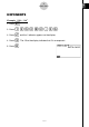
11 Quick-Start TABLE FUNCTION The Table Function makes it possible to generate a table of solutions as different values are assigned to the variables of a function. Example: To create a number table for the following function Y = X (X+1) (X–2) 1. Press 2. Use m. defc to highlight w. TABLE, and then press 3. Input the formula. v(v+b) (v-c)w 4. Press table.
Precautions when Using this Product A progress bar and/or a busy indicator appear on the display whenever the calculator is performing a calculation, writing to memory (including Flash memory), or reading from memory (including Flash memory). Busy indicator Progress bar Never press the P button or remove the batteries from the calculator when the progress bar or busy indicator is on the display. Doing so can cause memory contents to be lost and can cause malfunction of the calculator.
Handling Precautions • Your calculator is made up of precision components. Never try to take it apart. • Avoid dropping your calculator and subjecting it to strong impact. • Do not store the calculator or leave it in areas exposed to high temperatures or humidity, or large amounts of dust. When exposed to low temperatures, the calculator may require more time to display results and may even fail to operate. Correct operation will resume once the calculator is brought back to normal temperature.
Be sure to keep physical records of all important data! Low battery power or incorrect replacement of the batteries that power the unit can cause the data stored in memory to be corrupted or even lost entirely. Stored data can also be affected by strong electrostatic charge or strong impact. It is up to you to keep back up copies of data to protect against its loss. In no event shall CASIO Computer Co., Ltd.
1 Contents Contents Getting Acquainted — Read This First! Chapter 1 Basic Operation 1-1 1-2 1-3 1-4 1-5 1-6 1-7 1-8 1-9 Chapter 2 2-1 2-2 2-3 2-4 2-5 2-6 2-7 2-8 Chapter 3 3-1 3-2 3-3 3-4 Chapter 4 4-1 4-2 4-3 4-4 Keys ................................................................................................. 1-1-1 Display .............................................................................................. 1-2-1 Inputting and Editing Calculations ........................................
2 Contents Chapter 5 5-1 5-2 5-3 5-4 5-5 5-6 5-7 5-8 5-9 5-10 5-11 Chapter 6 6-1 6-2 6-3 6-4 6-5 6-6 6-7 Chapter 7 7-1 7-2 7-3 7-4 7-5 7-6 7-7 7-8 Graphing Sample Graphs ................................................................................ 5-1-1 Controlling What Appears on a Graph Screen ................................. 5-2-1 Drawing a Graph .............................................................................. 5-3-1 Storing a Graph in Picture Memory .................................
3 Contents Chapter 8 8-1 8-2 8-3 8-4 8-5 8-6 8-7 8-8 Chapter 9 9-1 9-2 9-3 9-4 9-5 9-6 9-7 9-8 Chapter 10 10-1 10-2 10-3 10-4 10-5 Chapter 11 11-1 11-2 11-3 11-4 Chapter 12 12-1 12-2 12-3 12-4 12-5 12-6 12-7 Programming Basic Programming Steps ................................................................ 8-1-1 PRGM Mode Function Keys ............................................................. 8-2-1 Editing Program Contents ................................................................
4 Contents Chapter 13 13-1 13-2 13-3 Appendix 1 2 3 4 5 6 Using SD Cards (fx-9860G SD only) Using an SD Card ........................................................................ 13-1-1 Formatting an SD Card ................................................................ 13-2-1 SD Card Precautions during Use ................................................. 13-3-1 Error Message Table ........................................................................... α-1-1 Input Ranges ......................
0 Getting Acquainted — Read This First! About this User’s Guide u! x( ) The above indicates you should press ! and then x, which will input a symbol. All multiple-key input operations are indicated like this. Key cap markings are shown, followed by the input character or command in parentheses. u m EQUA This indicates you should first press m, use the cursor keys (f, c, d, e) to select the EQUA mode, and then press w.
0-1-1 Getting Acquainted uGraphs As a general rule, graph operations are shown on facing pages, with actual graph examples on the right hand page. You can produce the same graph on your calculator by performing the steps under the Procedure above the graph. Look for the type of graph you want on the right hand page, and then go to the page indicated for that graph. The steps under “Procedure” always use initial RESET settings.
Chapter Basic Operation 1-1 1-2 1-3 1-4 1-5 1-6 1-7 1-8 1-9 Keys Display Inputting and Editing Calculations Option (OPTN) Menu Variable Data (VARS) Menu Program (PRGM) Menu Using the Setup Screen Using Screen Capture When you keep having problems… 20050401 1
1-1-1 Keys 1-1 Keys 20050401
1-1-2 Keys k Key Table Page Page Page Page Page Page 5-11-1 5-2-7 5-2-1 5-10-1 5-11-9 1-2-3 1-4-1 1-6-1 1-5-1 1-7-1 1-2-1 2-4-7 2-4-5 2-4-7 2-4-5 2-4-5 2-4-5 2-4-4 2-4-4 2-4-4 2-4-5 2-4-5 2-4-4 2-4-4 2-4-4 2-4-10 2-4-12 2-4-7 2-4-7 10-3-13 10-3-12 2-4-10 2-4-11 2-1-1 2-1-1 1-1-3 1-1-3 Page 1-8-1 Page 1-3-5 Page 1-3-7 2-2-1 Page Page 1-3-2 1-3-1 1-3-7 3-1-2 2-6-2 2-1-1 2-1-1 2-1-1 2-1-1 2-8-11 2-4-4 2-1-1 20050401 2-2-5 2-1-1
1-1-3 Keys k Key Markings Many of the calculator’s keys are used to perform more than one function. The functions marked on the keyboard are color coded to help you find the one you need quickly and easily. Function Key Operation l 1 log 2 x 10 !l 3 B al The following describes the color coding used for key markings. Color # Key Operation Orange Press ! and then the key to perform the marked function. Red Press a and then the key to perform the marked function.
1-2-1 Display 1-2 Display k Selecting Icons This section describes how to select an icon in the Main Menu to enter the mode you want. u To select an icon 1. Press m to display the Main Menu. 2. Use the cursor keys (d, e, f, c) to move the highlighting to the icon you want. Currently selected icon 3. Press w to display the initial screen of the mode whose icon you selected. Here we will enter the STAT mode.
1-2-2 Display Icon Mode Name Description S • SHT (Spreadsheet) Use this mode to perform spreadsheet calculations. Each file contains a 26-column × 999-line spreadsheet. In addition to the calculator’s built-in commands and S • SHT mode commands, you can also perform statistical calculations and graph statistical data using the same procedures that you use in the STAT mode. GRAPH Use this mode to store graph functions and to draw graphs using the functions.
1-2-3 Display k About the Function Menu Use the function keys (1 to 6) to access the menus and commands in the menu bar along the bottom of the display screen. You can tell whether a menu bar item is a menu or a command by its appearance. • Next Menu Example: Selecting displays a menu of hyperbolic functions. • Command Input Example: Selecting inputs the sinh command. • Direct Command Execution Example: Selecting executes the DRAW command.
1-2-4 Display k Normal Display The calculator normally displays values up to 10 digits long. Values that exceed this limit are automatically converted to and displayed in exponential format. u How to interpret exponential format 1.2E+12 indicates that the result is equivalent to 1.2 × 10¹². This means that you should move the decimal point in 1.2 twelve places to the right, because the exponent is positive. This results in the value 1,200,000,000,000. 1.
1-2-5 Display k Special Display Formats This calculator uses special display formats to indicate fractions, hexadecimal values, and degrees/minutes/seconds values. u Fractions 12 ................. Indicates: 456 –––– 23 u Hexadecimal Values ................. Indicates: 0ABCDEF1(16), which equals 180150001(10) u Degrees/Minutes/Seconds ................. Indicates: 12° 34’ 56.
1-3-1 Inputting and Editing Calculations 1-3 Inputting and Editing Calculations Note • Unless specifically noted otherwise, all of the operations in this section are explained using the Linear input mode. k Inputting Calculations When you are ready to input a calculation, first press A to clear the display. Next, input your calculation formulas exactly as they are written, from left to right, and press w to obtain the result.
1-3-2 Inputting and Editing Calculations In the Linear input mode, pressing !D(INS) changes the cursor to ‘‘ ’’. The next function or value you input is overwritten at the location of ‘‘ ’’. Acga ddd!D(INS) s To abort this operation, press !D(INS) again. u To delete a step ○ ○ ○ ○ ○ Example To change 369 × × 2 to 369 × 2 Adgj**c dD In the insert mode, the D key operates as a backspace key. #The cursor is a vertical flashing line (I) when the insert mode is selected.
1-3-3 Inputting and Editing Calculations u To insert a step ○ ○ ○ ○ ○ Example To change 2.362 to sin2.362 Ac.
1-3-4 Inputting and Editing Calculations k Using Replay Memory The last calculation performed is always stored into replay memory. You can recall the contents of the replay memory by pressing d or e. If you press e, the calculation appears with the cursor at the beginning. Pressing d causes the calculation to appear with the cursor at the end. You can make changes in the calculation as you wish and then execute it again. ○ ○ ○ ○ ○ Example 1 To perform the following two calculations 4.12 × 6.4 = 26.368 4.
1-3-5 Inputting and Editing Calculations k Making Corrections in the Original Calculation ○ ○ ○ ○ ○ Example 14 ÷ 0 × 2.3 entered by mistake for 14 ÷ 10 × 2.3 Abe/a*c.d w Press J. Cursor is positioned automatically at the location of the cause of the error. Make necessary changes. db Execute again. w k Using the Clipboard for Copy and Paste You can copy (or cut) a function, command, or other input to the clipboard, and then paste the clipboard contents at another location.
1-3-6 Inputting and Editing Calculations 3. Press 1(COPY) to copy the highlighted text to the clipboard, and exit the copy range specification mode. The selected characters are not changed when you copy them. To cancel text highlighting without performing a copy operation, press J. Math input mode 1. Use the cursor keys to move the cursor to the line you want to copy. 2. Press !i(CLIP) . The cursor will change to “ ”. 3. Press 1(CPY • L) to copy the highlighted text to the clipboard.
1-3-7 Inputting and Editing Calculations u Pasting Text Move the cursor to the location where you want to paste the text, and then press ! j(PASTE). The contents of the clipboard are pasted at the cursor position. A !j(PASTE) k Catalog Function The Catalog is an alphabetic list of all the commands available on this calculator. You can input a command by calling up the Catalog and then selecting the command you want. u To use the Catalog to input a command 1.
1-3-8 Inputting and Editing Calculations k Input Operations in the Math Input Mode Selecting “Math” for the “Input Mode” setting on the Setup screen (page 1-7-1) turns on the Math input mode, which allows natural input and display of certain functions, just as they appear in your textbook. Note • The initial default “Input Mode” setting is “Linear” (Linear input mode). Before trying to perform any of the operations explained in this section, be sure to change the “Input Mode” setting to “Math”.
1-3-9 Inputting and Editing Calculations u Math Input Mode Functions and Symbols The functions and symbols listed below can be used for natural input in the Math input mode. The “Bytes” column shows the number of bytes of memory that are used up by input in the Math input mode.
1-3-10 Inputting and Editing Calculations u Using the MATH Menu In the RUN • MAT mode, pressing 4(MATH) displays the MATH menu. You can use this menu for natural input of matrices, differentials, integrals, etc. • {MAT} ... {displays the MAT submenu, for natural input of matrices} • {2×2} ... {inputs a 2 × 2 matrix} • {3×3} ... {inputs a 3 × 3 matrix} • {m×n} ... {inputs a matrix with m lines and n columns (up to 6 × 6)} • {logab} ... {starts natural input of logarithm log ab} • {Abs} ...
1-3-11 Inputting and Editing Calculations ○ ○ ○ ○ ○ Example 2 ( 2 To input 1+ 5 A(b+ ) 2 $ cc f e )x w J ○ ○ ○ ○ ○ Example 3 1 To input 1+ 0 x + 1dx Ab+4(MATH)6(g)1(∫dx) a+(X)+b ea fb e w J 20050401
1-3-12 Inputting and Editing Calculations ○ ○ ○ ○ ○ Example 4 To input 2 × 1 2 2 2 1 2 Ac*4(MATH)1(MAT)1(2×2) $bcc ee !x( )ce e!x( )cee$bcc w u When the calculation does not fit within the display window Arrows appear at the left, right, top, or bottom edge of the display to let you know when there is more of the calculation off the screen in the corresponding direction. When you see an arrow, you can use the cursor keys to scroll the screen contents and view the part you want.
1-3-13 Inputting and Editing Calculations u Inserting a Function into an Existing Expression In the Math input mode, you can make insert a natural input function into an existing expression. Doing so will cause the value or parenthetical expression to the right of the cursor to become the argument of the inserted function. Use !D(INS) to insert a function into an existing expression.
1-3-14 Inputting and Editing Calculations u Functions that Support Insertion The following lists the functions that can be inserted using the procedure under “To insert a function into an existing expression” (page 1-3-13). It also provides information about how insertion affects the existing calculation.
1-3-15 Inputting and Editing Calculations • Note the following cursor operations you can use while inputting a calculation with natural display format. To do this: Move the cursor from the end of the calculation to the beginning Move the cursor from the beginning of the calculation to the end Press this key: e d u Math Input Mode Calculation Result Display Fractions, matrices, and lists produced by Math input mode calculations are displayed in natural format, just as they appear in your textbook.
1-3-16 Inputting and Editing Calculations u Math Input Mode Input Restrictions Note the following restrictions that apply during input of the Math input mode. • Certain types of expressions can cause the vertical width of a calculation formula to be greater than one display line. The maximum allowable vertical width of a calculation formula is about two display screens (120 dots). You cannot input any expression that exceeds this limitation.
1-4-1 Option (OPTN) Menu 1-4 Option (OPTN) Menu The option menu gives you access to scientific functions and features that are not marked on the calculator’s keyboard. The contents of the option menu differ according to the mode you are in when you press the K key. See “8-7 PRGM Mode Command List” for details on the option (OPTN) menu. u Option menu in the RUN • MAT or PRGM mode • {LIST} ... {list function menu} • {MAT} ... {matrix operation menu} • {CPLX} ... {complex number calculation menu} • {CALC} ..
1-4-2 Option (OPTN) Menu u Option menu during numeric data input in the STAT, TABLE, RECUR, EQUA and S • SHT modes • {LIST}/{CPLX}/{CALC}/{HYP}/{PROB}/{NUM}/{ANGL}/{ESYM}/{FMEM}/{LOGIC} u Option menu during formula input in the GRAPH, DYNA, TABLE, RECUR and EQUA modes • {List}/{CALC}/{HYP}/{PROB}/{NUM}/{FMEM}/{LOGIC} The following shows the function menus that appear under other conditions.
1-5-1 Variable Data (VARS) Menu 1-5 Variable Data (VARS) Menu To recall variable data, press J to display the variable data menu. {V-WIN}/{FACT}/{STAT}/{GRPH}/{DYNA}/ {TABL}/{RECR}/{EQUA*1}/{TVM*1} See “8-7 PRGM Mode Command List” for details on the variable data (VARS) menu. u V-WIN — Recalling V-Window values • {X}/{Y}/{T,θ } ... {x-axis menu}/{y-axis menu}/{T, θ menu} • {R-X}/{R-Y}/{R-T,θ } ... {x-axis menu}/{y-axis menu}/{T,θ menu} for right side of Dual Graph • {min}/{max}/{scal}/{dot}/{ptch} ...
1-5-2 Variable Data (VARS) Menu u STAT — Recalling statistical data • {X} … {single-variable, paired-variable x-data} • {n }/{o }/{Σ x }/{Σ x 2 }/{x σn }/{x σ n –1 }/{minX}/{maxX} …{number of data}/{mean}/{sum}/{sum of squares}/{population standard deviation}/{sample standard deviation}/{minimum value}/{maximum value} • {Y} ...
1-5-3 Variable Data (VARS) Menu u GRPH — Recalling Graph Functions • {Y}/{r} ... {rectangular coordinate or inequality function}/{polar coordinate function} • {Xt}/{Yt} ... parametric graph function {Xt}/{Yt} • {X} ... {X=constant graph function} (Press these keys before inputting a value to specify a storage memory.) u DYNA — Recalling Dynamic Graph Set Up Data • {Strt}/{End}/{Pitch} ...
1-5-4 Variable Data (VARS) Menu u RECR — Recalling Recursion Formula*1, Table Range, and Table Content Data • {FORM} ... {recursion formula data menu} • {an}/{an+1}/{an+2}/{bn}/{bn+1}/{bn+2}/{cn}/{cn+1}/{cn+2} ... {an}/{an+1}/{an+2}/{bn}/{bn+1}/{bn+2}/{cn}/{cn+1}/{cn+2} expressions • {RANG} ... {table range data menu} • {Strt}/{End} ... table range {start value}/{end value} • {a0}/{a1}/{a2}/{b0}/{b1}/{b2}/{c0}/{c1}/{c2} ... {a 0}/{a1}/{a2}/{b 0}/{b1}/{b2}/{c0}/{c1}/{c2} value • {anSt}/{bnSt}/{cnSt} ...
1-6-1 Program (PRGM) Menu 1-6 Program (PRGM) Menu To display the program (PRGM) menu, first enter the RUN • MAT or PRGM mode from the Main Menu and then press !J(PRGM). The following are the selections available in the program (PRGM) menu. • {COM} ...... {program command menu} • {CTL} ........ {program control command menu} • {JUMP} .... {jump command menu} • {? } ............ {input prompt} • {^} ........... {output command} • {CLR } ....... {clear command menu} • {DISP } ......
1-7-1 Using the Setup Screen 1-7 Using the Setup Screen The mode’s Setup screen shows the current status of mode settings and lets you make any changes you want. The following procedure shows how to change a setup. u To change a mode setup 1. Select the icon you want and press w to enter a mode and display its initial screen. Here we will enter the RUN • MAT mode. 2. Press !m(SET UP) to display the mode’s Setup screen. ... • This Setup screen is just one possible example.
1-7-2 Using the Setup Screen u Mode (calculation/binary, octal, decimal, hexadecimal mode) • {Comp} ... {arithmetic calculation mode} • {Dec}/{Hex}/{Bin}/{Oct} ... {decimal}/{hexadecimal}/{binary}/{octal} u Frac Result (fraction result display format) • {d/c}/{ab/c}... {improper}/{mixed} fraction u Func Type (graph function type) Pressing one of the following function keys also switches the function of the v key. • {Y=}/{r=}/{Parm}/{X=c} ...
1-7-3 Using the Setup Screen u Axes (graph axis display) • {On}/{Off} ... {display on}/{display off} u Label (graph axis label display) • {On}/{Off} ... {display on}/{display off} u Display (display format) • {Fix}/{Sci}/{Norm}/{Eng} ... {fixed number of decimal places specification}/{number of significant digits specification}/{normal display setting}/{engineering mode} u Stat Wind (statistical graph V-Window setting method) • {Auto}/{Man} ...
1-7-4 Using the Setup Screen u Background (graph display background) • {None}/{PICT} ... {no background}/{graph background picture specification} u Sketch Line (overlaid line type) •{ }/{ }{ }/{ } ... {normal}/{thick}/{broken}/{dot} u Dynamic Type (dynamic graph type) • {Cnt}/{Stop} ... {non-stop (continuous)}/{automatic stop after 10 draws} u Locus (dynamic graph locus mode) • {On}/{Off} ... {locus drawn}/{locus not drawn} u Y=Draw Speed (dynamic graph draw speed) • {Norm}/{High} ...
1-7-5 Using the Setup Screen u Date Mode (number of days per year setting) • {365}/{360} ... interest calculations using {365}*1/{360} days per year u Auto Calc (spreadsheet auto calc) • {On}/{Off} ... {execute}/{not execute} the formulas automatically u Show Cell (spreadsheet cell display mode) • {Form}/{Val} ... {formula}*2/{value} u Move (spreadsheet cell cursor direction)*3 • {Low}/{Right} ... {move down}/{move right} *1 The 365-day year must be used for date calculations in the TVM mode.
1-8-1 Using Screen Capture 1-8 Using Screen Capture Any time while operating the calculator, you can capture an image of the current screen and save it in capture memory. u To capture a screen image 1. Operate the calculator and display the screen you want to capture. 2. Press !h(CAPTURE). • This displays a memory area selection dialog box. 3. Input a value from 1 to 20 and then press w. • This will capture the screen image and save it in capture memory area named “Capt n” (n = the value you input).
1-9-1 When you keep having problems… 1-9 When you keep having problems… If you keep having problems when you are trying to perform operations, try the following before assuming that there is something wrong with the calculator. k Getting the Calculator Back to its Original Mode Settings 1. From the Main Menu, enter the SYSTEM mode. 2. Press 5(RSET). 3. Press 1(STUP), and then press 1(Yes). 4. Press Jm to return to the Main Menu.
1-9-2 When you keep having problems… k Low Battery Message If either of the following messages appears on the display, immediately turn off the calculator and replace main batteries as instructed. If you continue using the calculator without replacing main batteries, power will automatically turn off to protect memory contents. Once this happens, you will not be able to turn power back on, and there is the danger that memory contents will be corrupted or lost entirely.
Chapter Manual Calculations 2-1 2-2 2-3 2-4 2-5 2-6 2-7 2-8 Basic Calculations Special Functions Specifying the Angle Unit and Display Format Function Calculations Numerical Calculations Complex Number Calculations Binary, Octal, Decimal, and Hexadecimal Calculations with Integers Matrix Calculations Linear/Math input mode (page 1-3-8) • Unless specifically noted otherwise, all of the operations in this chapter are explained using the Linear input mode.
2-1-1 Basic Calculations 2-1 Basic Calculations k Arithmetic Calculations • Enter arithmetic calculations as they are written, from left to right. • Use the - key to input the minus sign before a negative value. • Calculations are performed internally with a 15-digit mantissa. The result is rounded to a 10-digit mantissa before it is displayed. • For mixed arithmetic calculations, multiplication and division are given priority over addition and subtraction. Example Operation 23 + 4.5 – 53 = –25.5 23+4.
2-1-2 Basic Calculations k Number of Decimal Places, Number of Significant Digits, Normal Display Range [SET UP]- [Display] -[Fix] / [Sci] / [Norm] • Even after you specify the number of decimal places or the number of significant digits, internal calculations are still performed using a 15-digit mantissa, and displayed values are stored with a 10-digit mantissa.
2-1-3 Basic Calculations Example 200 ÷ 7 × 14 = 400 Condition 3 decimal places Operation Display 200/7*14w 400 !m(SET UP) f (or c 12 times) 1(Fix)dwJw 400.000 200/7w * 14w 28.571 Ans × I 400.000 Calculation continues using display capacity of 10 digits • If the same calculation is performed using the specified number of digits: The value stored internally is rounded off to the number of decimal places specified on the Setup screen. 200/7w 28.571 K6(g)4(NUM)4(Rnd)w * 14w 28.
2-1-4 Basic Calculations 2 Type B functions With these functions, the value is entered and then the function key is pressed. x2, x–1, x!, ° ’ ”, ENG symbols, angle unit °, r, g 3 Power/root ^(xy), x' 4 Fractions a b/c 5 Abbreviated multiplication format in front of π, memory name, or variable name. 2π, 5A, etc. 6 Type C functions With these functions, the function key is pressed and then the value is entered.
2-1-5 Basic Calculations k Multiplication Operations without a Multiplication Sign You can omit the multiplication sign (×) in any of the following operations. • Before Type A functions (1 on page 2-1-3) and Type C functions (6 on page 2-1-4), except for negative signs Example 3, 2Pol(5, 12), etc. 2sin30, 10log1.2, 2' • Before constants, variable names, memory names Example 2π, 2AB, 3Ans, 3Y1, etc. • Before an open parenthesis Example 3(5 + 6), (A + 1)(B – 1), etc.
2-1-6 Basic Calculations • When you try to perform a calculation that causes memory capacity to be exceeded (Memory ERROR). • When you use a command that requires an argument, without providing a valid argument (Argument ERROR). • When an attempt is made to use an illegal dimension during matrix calculations (Dimension ERROR). • When you are in the real mode and an attempt is made to perform a calculation that produces a complex number solution.
2-2-1 Special Functions 2-2 Special Functions k Calculations Using Variables Example Operation Display 193.2aav(A)w 193.2 193.2 ÷ 23 = 8.4 av(A)/23w 8.4 193.2 ÷ 28 = 6.9 av(A)/28w 6.9 k Memory u Variables (Alpha Memory) This calculator comes with 28 variables as standard. You can use variables to store values you want to use inside of calculations. Variables are identified by single-letter names, which are made up of the 26 letters of the alphabet, plus r and θ.
2-2-2 Special Functions u To display the contents of a variable ○ ○ ○ ○ ○ Example To display the contents of variable A Aav(A)w u To clear a variable ○ ○ ○ ○ ○ Example To clear variable A Aaaav(A)w u To assign the same value to more than one variable [value]a [first variable name*1]a3(~) [last variable name*1]w ○ ○ ○ ○ ○ Example To assign a value of 10 to variables A through F Abaaav(A) a3(~)at(F)w u Function Memory [OPTN]-[FMEM] Function memory (f1~f20) is convenient for temporary storage of of
2-2-3 Special Functions u To store a function ○ ○ ○ ○ ○ Example To store the function (A+B) (A–B) as function memory number 1 (av(A)+al(B)) (av(A)-al(B)) K6(g)6(g)3(FMEM) 1(STO)bw JJJ u To recall a function ○ ○ ○ ○ ○ Example To recall the contents of function memory number 1 K6(g)6(g)3(FMEM) 2(RCL)bw u To recall a function as a variable daav(A)w baal(B)w K6(g)6(g)3(FMEM)3(fn) b+cw u To display a list of available functions K6(g)6(g)3(FMEM) 4(SEE) # If the function memory number to which you store a
2-2-4 Special Functions u To delete a function ○ ○ ○ ○ ○ Example To delete the contents of function memory number 1 AK6(g)6(g)3(FMEM) 1(STO)bw • Executing the store operation while the display is blank deletes the function in the function memory you specify. u To use stored functions ○ ○ ○ ○ ○ Example To store x3 + 1, x2 + x into function memory, and then graph: y = x3 + x2 + x + 1 Use the following V-Window settings.
2-2-5 Special Functions k Answer Function The Answer Function automatically stores the last result you calculated by pressing w (unless the w key operation results in an error). The result is stored in the answer memory. u To use the contents of the answer memory in a calculation Example 123 + 456 = 579 789 – 579 = 210 Abcd+efgw hij-!-(Ans)w In the Math input mode, the answer memory is refreshed with each calculation.
2-2-6 Special Functions k History Function The history function maintains a history of calculation expressions and results in the Math input mode. Up to 30 sets of calculation expressions and results are maintained. b+cw *cw You can also edit the calculation expressions that are maintained by the history function and recalculate. This will recalculate all of the expressions starting from the edited expression.
2-2-7 Special Functions k Stacks The unit employs memory blocks, called stacks, for storage of low priority values and commands. There is a 10-level numeric value stack, a 26-level command stack, and a 10level program subroutine stack. An error occurs if you perform a calculation so complex that it exceeds the capacity of available numeric value stack or command stack space, or if execution of a program subroutine exceeds the capacity of the subroutine stack.
2-2-8 Special Functions k Using Multistatements Multistatements are formed by connecting a number of individual statements for sequential execution. You can use multistatements in manual calculations and in programmed calculations. There are two different ways that you can use to connect statements to form multistatements. • Colon (:) Statements that are connected with colons are executed from left to right, without stopping.
2-3-1 Specifying the Angle Unit and Display Format 2-3 Specifying the Angle Unit and Display Format Before performing a calculation for the first time, you should use the Setup screen to specify the angle unit and display format. k Setting the Angle Unit [SET UP]- [Angle] 1. On the Setup screen, highlight “Angle”. 2. Press the function key for the angle unit you want to specify, then press J. • {Deg}/{Rad}/{Gra} ...
2-3-2 Specifying the Angle Unit and Display Format u To specify the number of significant digits (Sci) ○ ○ ○ ○ ○ Example To specify three significant digits 2(Sci) dw Press the number key that corresponds to the number of significant digits you want to specify (n = 0 to 9). Specifying 0 makes the number of significant digits 10. u To specify the normal display (Norm 1/Norm 2) Press 3(Norm) to switch between Norm 1 and Norm 2. Norm 1: 10–2 (0.01)>|x|, |x| >1010 Norm 2: 10–9 (0.
2-4-1 Function Calculations 2-4 Function Calculations k Function Menus This calculator includes five function menus that give you access to scientific functions not printed on the key panel. • The contents of the function menu differ according to the mode you entered from the Main Menu before you pressed the K key. The following examples show function menus that appear in the RUN • MAT mode. u Hyperbolic Calculations (HYP) [OPTN]-[HYP] • {sinh}/{cosh}/{tanh} ...
2-4-2 Function Calculations u Angle Units, Coordinate Conversion, Sexagesimal Operations (ANGL) [OPTN]-[ANGL] • {°}/{r}/{g} ... {degrees}/{radians}/{grads} for a specific input value • {° ’ ”} ... {specifies degrees (hours), minutes, seconds when inputting a degrees/minutes/ seconds value} • {° ’ ” } ... {converts decimal value to degrees/minutes/seconds value}*1 • {Pol(}/{Rec(} ... {rectangular-to-polar}/{polar-to-rectangular} coordinate conversion • {'DMS} ...
2-4-3 Function Calculations k Angle Units To change the angle unit of an input value, first press K6(g)5(ANGL). On the function key menu that appears, select “ ”, “r”, or “g”. ° • Be sure to specify Comp for Mode in the Setup screen. Example Operation To convert 4.25 rad to degrees: 243.5070629 !m(SET UP)cccccc1(Deg)J 4.25K6(g)5(ANGL)2(r)w 47.3° + 82.5rad = 4774.20181° 47.3+82.
2-4-4 Function Calculations k Trigonometric and Inverse Trigonometric Functions • Be sure to set the angle unit before performing trigonometric function and inverse trigonometric function calculations. π (90° = ––– radians = 100 grads) 2 • Be sure to specify Comp for Mode in the Setup screen. Example sin 63° = 0.8910065242 π cos (–– rad) = 0.5 3 Operation !m(SET UP)cccccc 1(Deg)J s63w !m(SET UP)cccccc 2(Rad)J c(!E(π)/3)w
2-4-5 Function Calculations k Logarithmic and Exponential Functions • Be sure to specify Comp for Mode in the Setup screen. Example Operation log 1.23 (log101.23) = 0.08990511144 l1.23w log2 8 = 3 K4(CALC)6(g)4(logab)2,8)w
2-4-6 Function Calculations k Hyperbolic and Inverse Hyperbolic Functions • Be sure to specify Comp for Mode in the Setup screen. Example Operation sinh 3.6 = 18.28545536 K6(g)2(HYP)1(sinh)3.6w cosh 1.5 – sinh 1.5 = 0.2231301601 = e –1.5 (Display: –1.5) K6(g)2(HYP)2(cosh)1.51(sinh)1.5w I!-(Ans)w (Proof of cosh x ± sinh x = e±x) cosh–1 20 15 = 0.7953654612 K6(g)2(HYP)5(cosh–1)(20/15)w
2-4-7 Function Calculations k Other Functions • Be sure to specify Comp for Mode in the Setup screen. Example Operation 2 + 5 = 3.65028154 !x( )2+!x( (3 + i) = 1.755317302 +0.2848487846i !x( )(d+!a(i))w
2-4-8 Function Calculations k Random Number Generation (Ran#) This function generates a 10-digit truly random or sequentially random number that is greater than zero and less than 1. • A truly random number is generated if you do not specify anything for the argument. Example Operation Ran# (Generates a random number.) K6(g)3(PROB)4(Ran#)w (Each press of w generates a new random number.) w w • Specifying an argument from 1 to 9 generates random numbers based on that sequence.
2-4-9 Function Calculations k Coordinate Conversion u Rectangular Coordinates u Polar Coordinates • With polar coordinates, θ can be calculated and displayed within a range of –180°< θ < 180° (radians and grads have same range). • Be sure to specify Comp for Mode in the Setup screen. Example Operation Calculate r and θ ° when x = 14 and y = 20.7 1 24.989 → 24.98979792 (r) 2 55.928 → 55.92839019 (θ) !m(SET UP)cccccc 1(Deg)J K6(g)5(ANGL)6(g)1(Pol() 14,20.
2-4-10 Function Calculations k Permutation and Combination u Permutation u Combination n! nPr = ––––– (n – r)! n! nCr = ––––––– r! (n – r)! • Be sure to specify Comp for Mode in the Setup screen.
2-4-11 Function Calculations • Be sure to specify Comp for Mode in the Setup screen. Example Operation
2-4-12 Function Calculations Switching between improper fraction and mixed fraction format Pressing the !M(<) key toggles the display fraction between mixed fraction and improper fraction format. Switching between fraction and decimal format ⇒ M ⇐ • If the calculation result includes a fraction, the display format (improper fraction or mixed fraction) is in accordance with the “Frac Result” setting of the Setup screen. For details, see “1-7 Using the Setup Screen”.
2-5-1 Numerical Calculations 2-5 Numerical Calculations The following describes the items that are available in the menus you use when performing differential/quadratic differential, integration, Σ, maximum/minimum value, and Solve calculations. When the option menu is on the display, press 4(CALC) to display the function analysis menu. The items of this menu are used when performing specific types of calculations. • {Solve}/{d/dx}/{d2/dx2}/{∫dx}/{FMin}/{FMax}/{Σ(} ...
2-5-2 Numerical Calculations k Differential Calculations [OPTN]-[CALC]-[d /dx] To perform differential calculations, first display the function analysis menu, and then input the values using the syntax below.
2-5-3 Numerical Calculations Example To determine the derivative at point x = 3 for the function y = x3 + 4x2 + x – 6, with a tolerance of “tol” = 1E – 5 Input the function f(x). AK4(CALC)2(d/dx)vMd+evx+v-g, Input point x = a for which you want to determine the derivative. d, Input the tolerance value. bE-f) w
2-5-4 Numerical Calculations u Applications of Differential Calculations • Differentials can be added, subtracted, multiplied or divided with each other. d d ––– f (a) = f '(a), ––– g (a) = g'(a) dx dx Therefore: f '(a) + g'(a), f '(a) × g'(a), etc. • Differential results can be used in addition, subtraction, multiplication, and division, and in functions. 2 × f '(a), log ( f '(a)), etc. • Functions can be used in any of the terms ( f (x), a, tol) of a differential. d ––– (sinx + cosx, sin0.
2-5-5 Numerical Calculations [OPTN]-[CALC]-[d2/dx2] k Quadratic Differential Calculations After displaying the function analysis menu, you can input quadratic differentials using the following syntax.
2-5-6 Numerical Calculations
2-5-7 Numerical Calculations k Integration Calculations [OPTN]-[CALC]-[∫dx] To perform integration calculations, first display the function analysis menu and then input the values using the syntax below.
2-5-8 Numerical Calculations
2-5-9 Numerical Calculations Note the following points to ensure correct integration values. (1) When cyclical functions for integration values become positive or negative for different divisions, perform the calculation for single cycles, or divide between negative and positive, and then add the results together.
2-5-10 Numerical Calculations k Σ Calculations [OPTN]-[CALC]-[Σ ] To perform Σ calculations, first display the function analysis menu, and then input the values using the syntax below. K4(CALC)6(g)3(Σ( ) a k , k , α , β , n ) β Σ (a , k, α, β, n) = Σ a = a k α k k=α + aα +1 +........+ aβ (n: distance between partitions) ○ ○ ○ ○ ○ Example To calculate the following: 6 Σ (k 2 – 3k + 5) k=2 Use n = 1 as the distance between partitions.
2-5-11 Numerical Calculations u Σ Calculation Applications • Arithmetic operations using Σ calculation expressions n n k=1 k=1 Sn = Σ ak, Tn = Σ bk Expressions: Sn + Tn, Sn – Tn, etc. Possible operations: • Arithmetic and function operations using Σ calculation results 2 × Sn, log (Sn), etc. • Function operations using Σ calculation terms (ak, k) Σ (sink, k, 1, 5), etc.
2-5-12 Numerical Calculations k Maximum/Minimum Value Calculations [OPTN]-[CALC]-[FMin]/[FMax] After displaying the function analysis menu, you can input maximum/minimum calculations using the formats below, and solve for the maximum and minimum of a function within interval a < x < b.
2-5-13 Numerical Calculations ○ ○ ○ ○ ○ Example 2 To determine the maximum value for the interval defined by start point a = 0 and end point b = 3, with a precision of n = 6 for the function y = –x2 + 2 x + 2 Input f(x). AK4(CALC)6(g)2(FMax) -vx+cv+c, Input the interval a = 0, b = 3. a,d, Input the precision n = 6. g) w # In the function f(x), only X can be used as a variable in expressions.
2-6-1 Complex Number Calculations 2-6 Complex Number Calculations You can perform addition, subtraction, multiplication, division, parentheses calculations, function calculations, and memory calculations with complex numbers just as you do with the manual calculations described on pages 2-1-1 and 2-4-7. You can select the complex number calculation mode by changing the Complex Mode item on the Setup screen to one of the following settings. • {Real} ...
2-6-2 Complex Number Calculations k Arithmetic Operations [OPTN]-[CPLX]-[i] Arithmetic operations are the same as those you use for manual calculations. You can even use parentheses and memory.
2-6-3 Complex Number Calculations k Absolute Value and Argument [OPTN]-[CPLX]-[Abs]/[Arg] The unit regards a complex number in the form a + bi as a coordinate on a Gaussian plane, and calculates absolute value Z and argument (arg).
2-6-4 Complex Number Calculations k Extraction of Real and Imaginary Parts [OPTN]-[CPLX]-[ReP]/[lmP] Use the following procedure to extract the real part a and the imaginary part b from a complex number of the form a + bi.
2-6-5 Complex Number Calculations k Polar and Rectangular Form Transformation [OPTN]-[CPLX]-[ 'r ∠θ ]/[ ' a +bi ] Use the following procedure to transform a complex number displayed in rectangular form to polar form, and vice versa.
2-7-1 Binary, Octal, Decimal, and Hexadecimal Calculations with Integers 2-7 Binary, Octal, Decimal, and Hexadecimal Calculations with Integers You can use the RUN • MAT mode and binary, octal, decimal, and hexadecimal settings to perform calculations that involve binary, octal, decimal and hexadecimal values. You can also convert between number systems and perform bitwise operations. • You cannot use scientific functions in binary, octal, decimal, and hexadecimal calculations.
2-7-2 Binary, Octal, Decimal, and Hexadecimal Calculations with Integers • The following are the calculation ranges for each of the number systems.
2-7-3 Binary, Octal, Decimal, and Hexadecimal Calculations with Integers k Selecting a Number System You can specify decimal, hexadecimal, binary, or octal as the default number system using the Setup screen. u To specify a number system for an input value You can specify a number system for each individual value you input. Press 1(d~o) to display a menu of number system symbols. Press the function key that corresponds to the symbol you want to select and then input the value. • {d}/{h}/{b}/{o} ...
2-7-4 Binary, Octal, Decimal, and Hexadecimal Calculations with Integers ○ ○ ○ ○ ○ Example 2 To input and execute 1238 × ABC16, when the default number system is decimal or hexadecimal !m(SET UP)c2(Dec)J A1(d~o)4(o)bcd* 2(h)ABC*1w J3(DISP)2('Hex)w k Negative Values and Bitwise Operations Press 2(LOG) to display a menu of negation and bitwise operators. • {Neg} ... {negation}*2 • {Not}/{and}/{or}/{xor}/{xnor} ...
2-7-5 Binary, Octal, Decimal, and Hexadecimal Calculations with Integers ○ ○ ○ ○ ○ Example 2 To display the result of “368 or 11102” as an octal value !m(SET UP)c5(Oct)J Adg2(LOG) 4(or)J1(d~o)3(b) bbbaw ○ ○ ○ ○ ○ Example 3 To negate 2FFFED16 !m(SET UP)c3(Hex)J A2(LOG)2(Not) cFFFED*1w u Number System Transformation Press 3(DISP) to display a menu of number system transformation functions. • {'Dec}/{'Hex}/{'Bin}/{'Oct} ...
2-8-1 Matrix Calculations 2-8 Matrix Calculations From the Main Menu, enter the RUN • MAT mode, and press 1('MAT) to perform Matrix calculations. 26 matrix memories (Mat A through Mat Z) plus a Matrix Answer Memory (MatAns), make it possible to perform the following matrix operations.
2-8-2 Matrix Calculations k Inputting and Editing Matrices Pressing 1('MAT) displays the Matrix Editor screen. Use the Matrix Editor to input and edit matrices. m × n … m (row) × n (column) matrix None… no matrix preset • {DEL}/{DEL·A} ... deletes {a specific matrix}/{all matrices} • {DIM} ... {specifies the matrix dimensions (number of cells)} u Creating a Matrix To create a matrix, you must first define its dimensions (size) in the Matrix Editor. Then you can input values into the matrix.
2-8-3 Matrix Calculations u To input cell values Example To input the following data into Matrix B : 1 2 3 4 5 6 The following operation is a continuation of the example calculation on the previous page. bwcwdw ewfwgw (Data is input into the highlighted cell. Each time you press w, the highlighting moves to the next cell to the right.) To exit the Matrix input screen, press J. # You cannot input complex numbers into the cell of a matrix.
2-8-4 Matrix Calculations u Deleting Matrices You can delete either a specific matrix or all matrices in memory. u To delete a specific matrix 1. While the Matrix Editor is on the display, use f and c to highlight the matrix you want to delete. 2. Press 1(DEL). 3. Press 1(Yes) to delete the matrix or 6(No) to abort the operation without deleting anything. u To delete all matrices 1. While the Matrix Editor is on the display, press 2(DEL·A). 2.
2-8-5 Matrix Calculations k Matrix Cell Operations Use the following procedure to prepare a matrix for cell operations. 1. While the Matrix Editor is on the display, use f and c to highlight the name of the matrix you want to use. You can jump to a specific matrix by inputting the letter that corresponds to the matrix name. Inputting ai(N), for example, jumps to Mat N. Pressing !-(Ans) jumps to the Matrix current Memory. 2. Press w and the function menu with the following items appears. • {R-OP} ...
2-8-6 Matrix Calculations u To calculate the scalar multiplication of a row ○ ○ ○ ○ ○ Example To calculate the product of row 2 of the following matrix and the scalar 4: Matrix A = 1 2 3 4 5 6 1(R-OP)2(×Rw) Input multiplier value. ew Specify row number.
2-8-7 Matrix Calculations u To add two rows together ○ ○ ○ ○ ○ Example To add row 2 to row 3 of the following matrix : Matrix A = 1 2 3 4 5 6 1(R-OP)4(Rw+) Specify number of row to be added. cw Specify number of row to be added to. dw 6(EXE) (or w) u Row Operations • { DEL} ... {delete row} • {INS} ... {insert row} • {ADD} ...
2-8-8 Matrix Calculations u To insert a row ○ ○ ○ ○ ○ Example To insert a new row between rows one and two of the following matrix : Matrix A = 1 2 3 4 5 6 c 2(ROW)2(INS) u To add a row ○ ○ ○ ○ ○ Example To add a new row below row 3 of the following matrix : Matrix A = 1 2 3 4 5 6 cc 2(ROW)3(ADD) 20050401
2-8-9 Matrix Calculations u Column Operations • {DEL} ... {delete column} • {INS} ... {insert column} • {ADD} ...
2-8-10 Matrix Calculations u To add a column ○ ○ ○ ○ ○ Example To add a new column to the right of column 2 of the following matrix : Matrix A = 1 2 3 4 5 6 e 3(COL)3(ADD) k Modifying Matrices Using Matrix Commands [OPTN]-[MAT] u To display the matrix commands 1. From the Main Menu, enter the RUN • MAT mode. 2. Press K to display the option menu. 3. Press 2(MAT) to display the matrix command menu.
2-8-11 Matrix Calculations u Matrix Data Input Format [OPTN]-[MAT]-[Mat] The following shows the format you should use when inputting data to create a matrix using the Mat command. a11 a12 a21 a22 a1n a2n am1 am2 amn = [ [a11, a12, ..., a1n] [a21, a22, ..., a2n] .... [am1, am2, ...
2-8-12 Matrix Calculations u To input an identity matrix [OPTN]-[MAT]-[Iden] Use the Identity command to create an identity matrix. ○ ○ ○ ○ ○ Example 2 To create a 3 × 3 identity matrix as Matrix A K2(MAT)6(g)1(Iden) da6(g)1(Mat)av(A)w Number of rows/columns u To check the dimensions of a matrix [OPTN]-[MAT]-[Dim] Use the Dim command to check the dimensions of an existing matrix.
2-8-13 Matrix Calculations u Modifying Matrices Using Matrix Commands You can also use matrix commands to assign values to and recall values from an existing matrix, to fill in all cells of an existing matrix with the same value, to combine two matrices into a single matrix, and to assign the contents of a matrix column to a list file.
2-8-14 Matrix Calculations u To fill a matrix with identical values and to combine two matrices into a single matrix [OPTN]-[MAT]-[Fill]/[Aug] Use the Fill command to fill all the cells of an existing matrix with an identical value and the Augment command to combine two existing matrices into a single matrix.
2-8-15 Matrix Calculations u To assign the contents of a matrix column to a list [OPTN]-[MAT]-[M→L] Use the following format with the Mat→List command to specify a column and a list.
2-8-16 Matrix Calculations k Matrix Calculations [OPTN]-[MAT] Use the matrix command menu to perform matrix calculation operations. u To display the matrix commands 1. From the Main Menu, enter the RUN • MAT mode. 2. Press K to display the option menu. 3. Press 2(MAT) to display the matrix command menu. The following describes only the matrix commands that are used for matrix arithmetic operations. • {Mat} ... {Mat command (matrix specification)} • {Det} ... {Det command (determinant command)} • {Trn} .
2-8-17 Matrix Calculations u Matrix Arithmetic Operations [OPTN]-[MAT]-[Mat]/[Iden] ○ ○ ○ ○ ○ Example 1 To add the following two matrices (Matrix A + Matrix B) : A= 1 1 2 1 B= 2 3 2 1 AK2(MAT)1(Mat)av(A)+ 1(Mat)al(B)w ○ ○ ○ ○ ○ Example 2 Calculate the product to the following matrix using a multiplier value of 5 : Matrix A = 1 2 3 4 AfK2(MAT)1(Mat) av(A)w ○ ○ ○ ○ ○ Example 3 To multiply the two matrices in Example 1 (Matrix A × Matrix B) AK2(MAT)1(Mat)av(A)* 1(Mat)al(B)w ○ ○ ○ ○ ○
2-8-18 Matrix Calculations u Determinant [OPTN]-[MAT]-[Det] ○ ○ ○ ○ ○ Example Obtain the determinant for the following matrix : 1 2 3 4 5 6 –1 –2 0 Matrix A = K2(MAT)3(Det)1(Mat) av(A)w u Matrix Transposition [OPTN]-[MAT]-[Trn] A matrix is transposed when its rows become columns and its columns become rows.
2-8-19 Matrix Calculations u Matrix Inversion [OPTN]-[MAT]-[x –1] ○ ○ ○ ○ ○ Example To invert the following matrix : Matrix A = 1 2 3 4 K2(MAT)1(Mat) av(A)!) (x–1) w u Squaring a Matrix [OPTN]-[MAT]-[x 2] ○ ○ ○ ○ ○ Example To square the following matrix : Matrix A = 1 2 3 4 K2(MAT)1(Mat)av(A)xw # Only square matrices (same number of rows and columns) can be inverted. Trying to invert a matrix that is not square produces an error.
2-8-20 Matrix Calculations u Raising a Matrix to a Power [OPTN]-[MAT]-[ ] ○ ○ ○ ○ ○ Example To raise the following matrix to the third power : Matrix A = 1 2 3 4 K2(MAT)1(Mat)av(A) Mdw u Determining the Absolute Value, Integer Part, Fraction Part, and Maximum Integer of a Matrix [OPTN]-[NUM]-[Abs]/[Frac]/[Int]/[Intg] ○ ○ ○ ○ ○ Example To determine the absolute value of the following matrix : Matrix A = 1 –2 –3 4 K6(g)4(NUM)1(Abs) K2(MAT)1(Mat)av(A)w # Determinants and inverse matrices are
2-8-21 Matrix Calculations k Performing Matrix Calculations Using Natural Input u To specify the dimensions (size) of a matrix 1. In the RUN • MAT mode, press !m(SET UP)1(Math)J. 2. Press 4(MATH) to display the MATH menu. 3. Press 1(MAT) to display the following menu. • {2×2} … {inputs a 2 × 2 matrix} • {3×3} … {inputs a 3 × 3 matrix} • {m×n} … {inputs an m-row × n-column matrix (up to 6 × 6)} ○ ○ ○ ○ ○ Example To create a 2-row × 3-column matrix 3(m×n) Specify the number of rows.
2-8-22 Matrix Calculations u To input cell values ○ ○ ○ ○ ○ Example To perform the calculation shown below 1 1 2 33 13 4 5 6 ×8 The following operation is a continuation of the example calculation on the previous page.
Chapter 3 List Function A list is a storage place for multiple data items. This calculator lets you store up to 26 lists in a single file, and you can store up to six files in memory. Stored lists can be used in arithmetic and statistical calculations, and for graphing. Element number List 1 SUB 1 2 3 4 5 6 7 8 • • • • 3-1 3-2 3-3 3-4 56 37 21 69 40 48 93 30 • • • • Display range Cell List 2 List 3 1 2 4 8 16 32 64 128 107 75 122 87 298 48 338 49 • • • • • • • • Column List 4 List 5 3.5 6 2.
3-1-1 Inputting and Editing a List 3-1 Inputting and Editing a List When you enter the STAT mode, the “List Editor” will appear first. You can use the List Editor to input data into a list and to perform a variety of other list data operations. u To input values one-by-one Use the cursor keys to move the highlighting to the list name, sub name or cell you want to select. The screen automatically scrolls when the highlighting is located at either edge of the screen.
3-1-2 Inputting and Editing a List u To batch input a series of values 1. Use the cursor keys to move the highlighting to another list. 2. Press !*( { ), and then input the values you want, pressing , between each one. Press !/( } ) after inputting the final value. !*( { )g,h,i!/( } ) 3. Press w to store all of the values in your list. w You can also use list names inside of a mathematical expression to input values into another cell.
3-1-3 Inputting and Editing a List k Editing List Values u To change a cell value Use the cursor keys to move the highlighting to the cell whose value you want to change. Input the new value and press w to replace the old data with the new one. u To edit the contents of a cell 1. Use the cursor keys to move the highlighting to the cell whose contents you want to edit. 2. Press 6(䉯)2(EDIT). 3. Make any changes in the data you want. u To delete a cell 1.
3-1-4 Inputting and Editing a List u To delete all cells in a list Use the following procedure to delete all the data in a list. 1. Use the cursor key to move the highlighting to any cell of the list whose data you want to delete. 2. Pressing 6(䉯)4(DEL • A) causes a confirmation message to appear. 3. Press 1(Yes) to delete all the cells in the selected list or 6(No) to abort the delete operation without deleting anything. u To insert a new cell 1.
3-1-5 Inputting and Editing a List k Naming a List You can assign List 1 through List 26 “sub names” of up to eight bytes each. u To name a list 1. On the Setup screen, highlight “Sub Name” and then press 1(On)J. 2. Use the cursor keys to move the highlighting to the SUB cell of the list you want to name. 3. Type in the name and then press w. • To type in a name using alpha characters, press !a to enter the ALPHA-LOCK mode.
3-1-6 Inputting and Editing a List k Sorting List Values You can sort lists into either ascending or descending order. The highlighting can be located in any cell of the list. u To sort a single list Ascending order 1. While the lists are on the screen, press 6(䉯)1(TOOL)1(SRT • A). 2. The prompt “How Many Lists?:” appears to ask how many lists you want to sort. Here we will input 1 to indicate we want to sort only one list. bw 3.
3-1-7 Inputting and Editing a List u To sort multiple lists You can link multiple lists together for a sort so that all of their cells are rearranged in accordance with the sorting of a base list. The base list is sorted into either ascending order or descending order, while the cells of the linked lists are arranged so that the relative relationship of all the rows is maintained. Ascending order 1. While the lists are on the screen, press 6(䉯)1(TOOL)1(SRT • A). 2.
3-1-8 Inputting and Editing a List Descending order Use the same procedure as that for the ascending order sort. The only difference is that you should press 2(SRT • D) in place of 1(SRT • A). # You can specify a value from 1 to 6 as the number of lists for sorting. # If you specify a list more than once for a single sort operation, an error occurs. An error also occurs if lists specified for sorting do not have the same number of values (rows).
3-2-1 Manipulating List Data 3-2 Manipulating List Data List data can be used in arithmetic and function calculations. In addition, various list data manipulation functions make manipulation of list data quick and easy. You can use list data manipulation functions in the RUN • MAT, STAT, TABLE, EQUA and PRGM modes. k Accessing the List Data Manipulation Function Menu All of the following examples are performed after entering the RUN • MAT mode.
3-2-2 Manipulating List Data u To count the number of data items in a list [OPTN]-[LIST]-[Dim] K1(LIST)3(Dim)1(List) w • The number of cells a list contains is its “dimension.” ○ ○ ○ ○ ○ Example To count the number of values in List 1 (36, 16, 58, 46, 56) AK1(LIST)3(Dim) 1(List)bw u To create a list or matrix by specifying the number of data items [OPTN]-[LIST]-[Dim] Use the following procedure to specify the number of data in the assignment statement and create a list.
3-2-3 Manipulating List Data ○ ○ ○ ○ ○ To create a 2-row × 3-column matrix (each cell of which contains 0) in Matrix A Example A!*( { )c,d!/( } )a K1(LIST)3(Dim) K2(MAT)1(Mat)av(A)w The following shows the new contents of Mat A. u To replace all data items with the same value [OPTN]-[LIST]-[Fill] K1(LIST)4(Fill) ,1(List) )w ○ ○ ○ ○ ○ Example To replace all data items in List 1 with the number 3 AK1(LIST)4(Fill) d,1(List)b)w The following shows the new contents of List 1.
3-2-4 Manipulating List Data u To find the minimum value in a list [OPTN]-[LIST]-[Min] K1(LIST)6(g)1(Min)6(g)6(g)1(List) )w ○ ○ ○ ○ ○ Example To find the minimum value in List 1 (36, 16, 58, 46, 56) AK1(LIST)6(g)1(Min) 6(g)6(g)1(List)b)w u To find the maximum value in a list [OPTN]-[LIST]-[Max] Use the same procedure as when finding the minimum value (Min), except press 6(g)2(Max) in place of 6(g)1(Min).
3-2-5 Manipulating List Data u To calculate the mean of data items [OPTN]-[LIST]-[Mean] K1(LIST)6(g)3(Mean)6(g)6(g)1(List) )w ○ ○ ○ ○ ○ Example To calculate the mean of data items in List 1 (36, 16, 58, 46, 56) AK1(LIST)6(g)3(Mean) 6(g)6(g)1(List)b)w u To calculate the mean of data items of specified frequency [OPTN]-[LIST]-[Mean] This procedure uses two lists: one that contains values and one that indicates the frequency (number of occurrences) of each value.
3-2-6 Manipulating List Data u To calculate the median of data items of specified frequency [OPTN]-[LIST]-[Med] This procedure uses two lists: one that contains values and one that indicates the frequency (number of occurrences) of each value. The frequency of the data in Cell 1 of the first list is indicated by the value in Cell 1 of the second list, etc. • The two lists must contain the same number of data items. If they don’t, an error occurs.
3-2-7 Manipulating List Data u To calculate the product of values in a list [OPTN]-[LIST]-[Prod] K1(LIST)6(g)6(g)2(Prod)6(g)1(List)w ○ ○ ○ ○ ○ Example To calculate the product of values in List 1 (2, 3, 6, 5, 4) AK1(LIST)6(g)6(g)2(Prod) 6(g)1(List)bw u To calculate the cumulative frequency of each data item [OPTN]-[LIST]-[Cuml] K1(LIST)6(g)6(g)3(Cuml)6(g)1(List) w • The result of this operation is stored in ListAns Memory.
3-2-8 Manipulating List Data ○ ○ ○ ○ ○ Example To calculate the percentage represented by each data item in List 1 (2, 3, 6, 5, 4) AK1(LIST)6(g)6(g)4(%) 6(g)1(List)bw 2/(2+3+6+5+4) × 100 = 3/(2+3+6+5+4) × 100 = 6/(2+3+6+5+4) × 100 = 5/(2+3+6+5+4) × 100 = 4/(2+3+6+5+4) × 100 = u To calculate the differences between neighboring data inside a list [OPTN]-[LIST]-[A A] K1(LIST)6(g)6(g)5(A)w • The result of this operation is stored in ListAns memory.
3-3-1 Arithmetic Calculations Using Lists 3-3 Arithmetic Calculations Using Lists You can perform arithmetic calculations using two lists or one list and a numeric value. List Numeric Value + − × ÷ ListAns Memory List = Numeric Value List Calculation results are stored in ListAns Memory. k Error Messages • A calculation involving two lists performs the operation between corresponding cells.
3-3-2 Arithmetic Calculations Using Lists u To directly input a list of values You can also directly input a list of values using {, }, and ,. ○ ○ ○ ○ ○ Example 1 To input the list: 56, 82, 64 !*( { )fg,ic, ge!/( } ) ○ ○ ○ ○ ○ Example 2 To multiply List 3 ( = 41 65 22 ) by the list 6 0 4 K1(LIST)1(List)d*!*( { )g,a,e!/( } )w The resulting list 246 0 is stored in ListAns Memory. 88 u To assign the contents of one list to another list Use a to assign the contents of one list to another list.
3-3-3 Arithmetic Calculations Using Lists u To recall the value in a specific list cell You can recall the value in a specific list cell and use it in a calculation. Specify the cell number by enclosing it inside square brackets. ○ ○ ○ ○ ○ Example To calculate the sine of the value stored in Cell 3 of List 2 sK1(LIST)1(List)c!+( [ )d!-( ] )w u To input a value into a specific list cell You can input a value into a specific list cell inside a list.
3-3-4 Arithmetic Calculations Using Lists k Graphing a Function Using a List When using the graphing functions of this calculator, you can input a function such as Y1 = List 1 X. If List 1 contains the values 1, 2, 3, this function will produces three graphs: Y = X, Y = 2X, Y = 3X. There are certain limitations on using lists with graphing functions. ○ ○ ○ ○ ○ Example To input the data 1, 2, 3 into List 1, and then graph the data in the GRAPH mode 1. In the STAT mode, input 1, 2, 3 into List 1. 2.
3-3-5 Arithmetic Calculations Using Lists 5. Press bw. 6. Enter the STAT mode to confirm that TABLE mode column Y1 has been copied to List 1. k Performing Scientific Function Calculations Using a List Lists can be used just as numeric values are in scientific function calculations. When the calculation produces a list as a result, the list is stored in ListAns Memory. ○ ○ ○ ○ ○ Example 41 To use List 3 65 to perform sin (List 3) 22 Use radians as the angle unit. sK1(LIST)1(List)dw –0.
3-4-1 Switching Between List Files 3-4 Switching Between List Files You can store up to 26 lists (List 1 to List 26) in each file (File 1 to File 6). A simple operation lets you switch between list files. u To switch between list files 1. From the Main Menu, enter the STAT mode. Press !m(SET UP) to display the STAT mode Setup screen. 2. Use c to highlight “List File”. 3. Press 1(FILE) and then input the number of the list file you want to use.
Chapter 4 Equation Calculations Your graphic calculator can perform the following three types of calculations: • Simultaneous linear equations • Quadratic and cubic equations • Solve calculations From the Main Menu, enter the EQUA mode. • {SIML} ... {linear equation with 2 to 6 unknowns} • {POLY} ... {degree 2 or 3 equation} • {SOLV} ...
4-1-1 Simultaneous Linear Equations 4-1 Simultaneous Linear Equations Description You can solve simultaneous linear equations with two to six unknowns. • Simultaneous Linear Equation with Two Unknowns: a1x1 + b1x2 = c1 a2x1 + b2x2 = c2 • Simultaneous Linear Equation with Three Unknowns: … a1x1 + b1x2 + c1x3 = d1 a2x1 + b2x2 + c2x3 = d2 a3x1 + b3x2 + c3x3 = d3 Set Up 1. From the Main Menu, enter the EQUA mode. Execution 2.
4-1-2 Simultaneous Linear Equations ○ ○ ○ ○ ○ To solve the following simultaneous linear equations for x, y, and z Example 4x + y – 2z = – 1 x + 6y + 3z = 1 – 5x + 4y + z = – 7 Procedure 1 m EQUA 2 1(SIML) 2(3) 3 ewbw-cw-bw bwgwdwbw -fwewbw-hw 4 1(SOLV) Result Screen # Internal calculations are performed using a 15digit mantissa, but results are displayed using a 10-digit mantissa and a 2-digit exponent.
4-2-1 Quadratic and Cubic Equations 4-2 Quadratic and Cubic Equations Description You can use this calculator to solve quadratic equations and cubic equations. • Quadratic Equation: ax2 + bx + c = 0 (a ≠ 0) • Cubic Equation: ax3 + bx2 + cx + d = 0 (a ≠ 0) Set Up 1. From the Main Menu, enter the EQUA mode. Execution 2. Select the POLY (higher degree equation) mode, and specify the degree of the equation. You can specify a degree 2 or 3. 3. Sequentially input the coefficients.
4-2-2 Quadratic and Cubic Equations ○ ○ ○ ○ ○ Example To solve the cubic equation (Angle unit = Rad) x3 – 2x2 – x + 2 = 0 Procedure 1 m EQUA 2 2(POLY) 2(3) 3 bw-cw-bwcw 4 1(SOLV) Result Screen Multiple Solutions (Example: x3 + 3x2 + 3x + 1 = 0) Complex Number Solution (Example: x3 + 2x2 + 3x + 2 = 0) Complex Mode: Real (page 1-7-2) Complex Mode: a + bi Complex Mode: r∠θ 20050401
4-3-1 Solve Calculations 4-3 Solve Calculations Description The Solve Calculation mode lets you determine the value of any variable in a formula without having to solve the equation. Set Up 1. From the Main Menu, enter the EQUA mode. Execution 2. Select the Solve Calculation mode, and input the equation as it is written. If you do not input an equals sign, the calculator assumes that the expression is to the left of the equals sign, and there is a zero to the right. *1 3.
4-3-2 Solve Calculations ○ ○ ○ ○ ○ Example An object thrown into the air at initial velocity V takes time T to reach height H. Use the following formula to solve for initial velocity V when H = 14 (meters), T = 2 (seconds) and gravitational acceleration is G = 9.8 (m/s2). H = VT – 1/2 GT2 Procedure 1 m EQUA 2 3(SOLV) aM(H)!.(=)ac(V)a/(T)-(b/c) a$(G)a/(T)xw 3 bew(H = 14) aw(V = 0) cw(T = 2) j.iw(G = 9.8) 4 Press fff to highlight V = 0, and then press 6(SOLV).
4-4-1 What to Do When an Error Occurs 4-4 What to Do When an Error Occurs u Error during coefficient value input Press the J key to clear the error and return to the value that was registered for the coefficient before you input the value that generated the error. Try inputting a new value again. u Error during calculation Press the J key to clear the error and display the coefficient. Try inputting values for the coefficients again. k Clearing Equation Memories 1.
Chapter 5 Graphing Sections 5-1 and 5-2 of this chapter provide basic information you need to know in order to draw a graph. The remaining sections describe more advanced graphing features and functions. Select the icon in the Main Menu that suits the type of graph you want to draw or the type of table you want to generate.
5-1-1 Sample Graphs 5-1 Sample Graphs k How to draw a simple graph (1) Description To draw a graph, simply input the applicable function. Set Up 1. From the Main Menu, enter the GRAPH mode. Execution 2. Input the function you want to graph. Here you would use the V-Window to specify the range and other parameters of the graph. See 5-2-1. 3. Draw the graph.
5-1-2 Sample Graphs ○ ○ ○ ○ ○ Example To graph y = 3x 2 Procedure 1 m GRAPH 2 dvxw 3 6(DRAW) (or w) Result Screen # Pressing A while a graph is on the display will return to the screen in step 2.
5-1-3 Sample Graphs k How to draw a simple graph (2) Description You can store up to 20 functions in memory and then select the one you want for graphing. Set Up 1. From the Main Menu, enter the GRAPH mode. Execution 2. Specify the function type and input the function whose graph you want to draw. You can use the GRAPH mode to draw a graph for the following types of expressions: rectangular coordinate expression, polar coordinate expression, parametric function, X = constant expression, inequality.
5-1-4 Sample Graphs ○ ○ ○ ○ ○ Example Input the functions shown below and draw their graphs Y1 = 2 x 2 – 3, r 2 = 3sin2θ Procedure 1 m GRAPH 2 3(TYPE)1(Y=)cvx-dw 3(TYPE)2(r=)dscvw 3 6(DRAW) Result Screen (Parametric) (Inequality) 20050401
5-1-5 Sample Graphs k How to draw a simple graph (3) Description Use the following procedure to graph the function of a parabola, circle, ellipse, or hyperbola. Set Up 1. From the Main Menu, enter the CONICS mode. Execution 2. Use the cursor fc keys to specify one of the function type as follows.
5-1-6 Sample Graphs ○ ○ ○ ○ ○ Example Graph the circle (X–1)2 + (Y–1)2 = 22 Procedure 1 m CONICS 2 ccccw 3 bwbwcw 4 6(DRAW) Result Screen (Parabola) (Ellipse) 20050401 (Hyperbola)
5-1-7 Sample Graphs k How to draw a simple graph (4) Description You can specify the graph line style, if you want. Set Up 1. From the Main Menu, enter the GRAPH mode. Execution 2. Input the function you want to graph. Here you would use the V-Window to specify the range and other parameters of the graph. See 5-2-1. 3. Select the line style. 4(STYL) 1( ) … Normal (initial default) 2( ) … Thick (twice the thickness of Normal) 3( ) … Broken (thick broken) 4( ) … Dot (dotted) 4. Draw the graph.
5-1-8 Sample Graphs ○ ○ ○ ○ ○ Example To graph y = 3x 2 Procedure 1 m GRAPH 2 3(TYPE)1(Y=)dvxw 3 f4(STYL)3( )J 4 6(DRAW) (or w) Result Screen (Normal) (Thick) 20050401 (Dotted)
5-2-1 Controlling What Appears on a Graph Screen 5-2 Controlling What Appears on a Graph Screen k V-Window (View Window) Settings Use the View Window to specify the range of the x- and y-axes, and to set the spacing between the increments on each axis. You should always set the V-Window parameters you want to use before graphing. u To make V-Window settings 1. From the Main Menu, enter the GRAPH mode. 2. Press !3(V-WIN) to display the V-Window setting screen.
5-2-2 Controlling What Appears on a Graph Screen u V-Window Setting Precautions • Inputting zero for Tθ ptch causes an error. • Any illegal input (out of range value, negative sign without a value, etc.) causes an error. • When Tθ max is less than Tθ min, Tθ ptch becomes negative. • You can input expressions (such as 2π) as V-Window parameters. • When the V-Window setting produces an axis that does not fit on the display, the scale of the axis is indicated on the edge of the display closest to the origin.
5-2-3 Controlling What Appears on a Graph Screen k Initializing and Standardizing the V-Window u To initialize the V-Window 1. From the Main Menu, enter the GRAPH mode. 2. Press !3(V-WIN). This displays the V-Window setting screen. 3. Press 1(INIT) to initialize the V-Window. Xmin = –6.3, Xmax = 6.3, Xscale = 1, Ymin = –3.1, Ymax = 3.1, Yscale = 1 Xdot = 0.
5-2-4 Controlling What Appears on a Graph Screen k V-Window Memory You can store up to six sets of V-Window settings in V-Window memory for recall when you need them. u To store V-Window settings 1. From the Main Menu, enter the GRAPH mode. 2. Press !3(V-WIN) to display the V-Window setting screen, and input the values you want. 3. Press 4(STO) to display the pop-up window. 4. Press a number key to specify the V-Window memory where you want to save the settings, and then press w.
5-2-5 Controlling What Appears on a Graph Screen k Specifying the Graph Range Description You can define a range (start point, end point) for a function before graphing it. Set Up 1. From the Main Menu, enter the GRAPH mode. 2. Make V-Window settings. Execution 3. Specify the function type and input the function. The following is the syntax for function input. Function ,!+( [ )Start Point , End Point !-( ] ) 4. Draw the graph.
5-2-6 Controlling What Appears on a Graph Screen ○ ○ ○ ○ ○ Example Graph y = x 2 + 3x – 2 within the range – 2 < x < 4 Use the following V-Window settings. Xmin = –3, Xmax = 5, Xscale = 1 Ymin = –10, Ymax = 30, Yscale = 5 Procedure 1 m GRAPH 2 !3(V-WIN) -dwfwbwc -bawdawfwJ 3 3(TYPE)1(Y=)vx+dv-c, !+( [ )-c,e!-( ] )w 4 6(DRAW) Result Screen # You can specify a range when graphing rectangular expressions, polar expressions, parametric functions, and inequalities.
5-2-7 Controlling What Appears on a Graph Screen k Zoom Description This function lets you enlarge and reduce the graph on the screen. Set Up 1. Draw the graph. Execution 2. Specify the zoom type. !2(ZOOM)1(BOX) ... Box zoom Draw a box around a display area, and that area is enlarged to fill the entire screen. 2(FACT) 3(IN)/4(OUT) ... Factor zoom The graph is enlarged or reduced in accordance with the factor you specify, centered on the current pointer location. 5(AUTO) ...
5-2-8 Controlling What Appears on a Graph Screen ○ ○ ○ ○ ○ Example Graph y = (x + 5)(x + 4)(x + 3), and then perform a box zoom. Use the following V-Window settings.
5-2-9 Controlling What Appears on a Graph Screen k Factor Zoom Description With factor zoom, you can zoom in or out, centered on the current cursor position. Set Up 1. Draw the graph. Execution 2. Press !2(ZOOM)2(FACT) to open a pop-up window for specifying the x-axis and y-axis zoom factor. Input the values you want and then press J. 3. Press !2(ZOOM)3(IN) to enlarge the graph, or !2(ZOOM)4(OUT) to reduce it. The graph is enlarged or reduced centered on the current pointer location. 4.
5-2-10 Controlling What Appears on a Graph Screen ○ ○ ○ ○ ○ Example Enlarge the graphs of the two expressions shown below five times on both the x - and y -axis to see if they are tangent. Y1 = (x + 4)(x + 1)(x – 3), Y2 = 3x + 22 Use the following V-Window settings.
5-3-1 Drawing a Graph 5-3 Drawing a Graph You can store up to 20 functions in memory. Functions in memory can be edited, recalled, and graphed. k Specifying the Graph Type Before you can store a graph function in memory, you must first specify its graph type. 1. While the Graph relation list is on the display, press 3(TYPE) to display the graph type menu, which contains the following items. • {Y=}/{r=}/{Parm}/{X=c} ... {rectangular coordinate}/{polar coordinate}/{parametric}/ {X=constant}*1 graph s} ...
5-3-2 Drawing a Graph u To store a polar coordinate function (r=) *1 ○ ○ ○ ○ ○ Example To store the following expression in memory area r2 : r = 5 sin3θ 3(TYPE)2(r=) (Specifies polar coordinate expression.) fsdv(Inputs expression.) w(Stores expression.) u To store a parametric function *2 ○ ○ ○ ○ ○ Example To store the following functions in memory areas Xt3 and Yt3 : x = 3 sin T y = 3 cos T 3(TYPE)3(Parm) (Specifies parametric expression.) dsvw(Inputs and stores x expression.
5-3-3 Drawing a Graph u To store an X = constant expression *1 ○ ○ ○ ○ ○ Example To store the following expression in memory area X4 : X=3 3(TYPE)4(X=c) (Specifies X = constant expression.) d(Inputs expression.) w(Stores expression.) • Inputting X, Y, T, r, or θ for the constant in the above procedures causes an error. u To store an inequality *1 ○ ○ ○ ○ ○ Example To store the following inequality in memory area Y5 : y > x2 – 2x – 6 3(TYPE)6(g)1(Y>) (Specifies an inequality.
5-3-4 Drawing a Graph u To assign values to the coefficients and variables of a graph function ○ ○ ○ ○ ○ Example To assign the values –1, 0, and 1 to variable A in Y = AX2–1, and draw a graph for each value 3(TYPE)1(Y=) av(A)vx-bw J4(GRPH)1(Y)b(av(A) !.(=)-b)w J4(GRPH)1(Y)b(av(A) !.(=)a)w J4(GRPH)1(Y)b(av(A) !.(=)b)w ffff1(SEL) 6(DRAW) The above three screens are produced using the Trace function. See “5-11 Function Analysis” for more information.
5-3-5 Drawing a Graph • If you do not specify a variable name (variable A in the above key operation), the calculator automatically uses one of the default variables listed below. Note that the default variable used depends on the memory area type where you are storing the graph function. Memory Area Type Default Variable Yn X rn θ Xtn T Ytn T fn X ○ ○ ○ ○ ○ Example Y1 (3) and Y1 (X = 3) are identical values.
5-3-6 Drawing a Graph k Editing and Deleting Functions u To edit a function in memory ○ ○ ○ ○ ○ Example To change the expression in memory area Y1 from y = 2x2 – 5 to y = 2x2 – 3 e (Displays cursor.) eeeeeDd(Changes contents.) w(Stores new graph function.) u To change the line style of a graph function 1. On the Graph relation list screen, use f and c to highlight the relation whose line style you want to change. 2. Press 4(STYL). 3. Select the line style.
5-3-7 Drawing a Graph u To change the type of a function*1 1. While the Graph relation list is on the display, press f or c to move the highlighting to the area that contains the function whose type you want to change. 2. Press 3(TYPE)5(CONV). 3. Select the function type you want to change to. ○ ○ ○ ○ ○ Example To change the function in memory area Y1 from y = 2x2 – 3 to y < 2x2 – 3 3(TYPE)5(CONV)3('Y<) (Changes the function type to “Y<”.) u To delete a function 1.
5-3-8 Drawing a Graph k Selecting Functions for Graphing u To specify the draw/non-draw status of a graph 1. On the graph relation list, use f and c to highlight the relation you do not want to graph. 2. Press 1(SEL). • Each press of 1(SEL) toggles graphing on and off. 3. Press 6(DRAW). Example To select the following functions for drawing : Y1 = 2x2 – 5, r2 = 5 sin3θ Use the following V-Window settings.
5-3-9 Drawing a Graph k Graph Memory Graph memory lets you store up to 20 sets of graph function data and recall it later when you need it. A single save operation saves the following data in graph memory. • All graph functions in the currently displayed Graph relation list (up to 20) • Graph types • Function graph line information • Draw/non-draw status • V-Window settings (1 set) u To store graph functions in graph memory 1. Press 5(GMEM)1(STO) to display the pop-up window. 2.
5-4-1 Storing a Graph in Picture Memory 5-4 Storing a Graph in Picture Memory You can save up to 20 graphic images in picture memory for later recall. You can overdraw the graph on the screen with another graph stored in picture memory. u To store a graph in picture memory 1. After graphing in GRAPH mode, press K1(PICT)1(STO) to display the pop-up window. 2. Press a number key to specify the Picture memory where you want to save the picture, and then press w.
5-5-1 Drawing Two Graphs on the Same Screen 5-5 Drawing Two Graphs on the Same Screen k Copying the Graph to the Sub-screen Description Dual Graph lets you split the screen into two parts. Then you can graph two different functions in each for comparison, or draw a normal size graph on one side and its enlarged version on the other side. This makes Dual Graph a powerful graph analysis tool.
5-5-2 Drawing Two Graphs on the Same Screen ○ ○ ○ ○ ○ Example Graph y = x(x + 1)(x – 1) in the main screen and sub-screen. Use the following V-Window settings. (Main Screen) Xmin = –2, Xmax = 2, Xscale = 0.5 Ymin = –2, Ymax = 2, Yscale = 1 Xmin = –4, Xmax = 4, Xscale = 1 Ymin = –3, Ymax = 3, Yscale = 1 (Sub-screen) Procedure 1 m GRAPH 2 !m(SET UP)cc1(G+G)J 3 !3(V-WIN) -cwcwa.
5-5-3 Drawing Two Graphs on the Same Screen k Graphing Two Different Functions Description Use the following procedure to graph different functions in the main screen and sub-screen. Set Up 1. From the Main Menu, enter the GRAPH mode. 2. On the Setup screen, select G+G for Dual Screen. 3. Make V-Window settings for the main screen. Press 6(RIGHT) to display the sub-graph settings screen. Pressing 6(LEFT) returns to the main screen setting screen. Execution 4.
5-5-4 Drawing Two Graphs on the Same Screen ○ ○ ○ ○ ○ Example Graph y = x(x + 1)(x – 1) in the main screen, and y = 2x2 – 3 in the subscreen. Use the following V-Window settings. (Main Screen) Xmin = –4, Xmax = 4, Xscale = 1 Ymin = –5, Ymax = 5, Yscale = 1 (Sub-screen) Xmin = –2, Xmax = 2, Xscale = 0.5 Ymin = –2, Ymax = 2, Yscale = 1 Procedure 1 m GRAPH 2 !m(SET UP)cc1(G+G)J 3 !3(V-WIN) -ewewbwc -fwfwbw 6(RIGHT) -cwcwa.
5-5-5 Drawing Two Graphs on the Same Screen k Using Zoom to Enlarge the Sub-screen Description Use the following procedure to enlarge the main screen graph and then move it to the subscreen. Set Up 1. From the Main Menu, enter the GRAPH mode. 2. On the Setup screen, select G+G for Dual Screen. 3. Make V-Window settings for the main screen. Execution 4. Input the function and draw the graph in the main screen. 5. Use Zoom to enlarge the graph, and then move it to the sub-screen.
5-5-6 Drawing Two Graphs on the Same Screen ○ ○ ○ ○ ○ Example Draw the graph y = x(x + 1)(x – 1) in the main screen, and then use Box Zoom to enlarge it. Use the following V-Window settings. (Main Screen) Xmin = –2, Xmax = 2, Xscale = 0.5 Ymin = –2, Ymax = 2, Yscale = 1 Procedure 1 m GRAPH 2 !m(SET UP)cc1(G+G)J 3 !3(V-WIN) -cwcwa.
5-6-1 Manual Graphing 5-6 Manual Graphing k Rectangular Coordinate Graph Description Inputting the Graph command in the RUN • MAT mode enables drawing of rectangular coordinate graphs. Set Up 1. From the Main Menu, enter the RUN • MAT mode. 2. Make V-Window settings. Execution 3. Input the commands for drawing the rectangular coordinate graph. 4. Input the function. # Certain functions can be graphed easily using built-in function graphs.
5-6-2 Manual Graphing ○ ○ ○ ○ ○ Example Graph y = 2 x 2 + 3 x – 4 Use the following V-Window settings.
5-6-3 Manual Graphing k Integration Graph Description Inputting the Graph command in the RUN • MAT mode enables graphing of functions produced by an integration calculation. The calculation result is shown in the lower left corner of the display, and the calculation range is cross plot type. Set Up 1. From the Main Menu, enter the RUN • MAT mode. 2. Make V-Window settings. Execution 3. Input graph commands for the integration graph. 4. Input the function.
5-6-4 Manual Graphing ○ ○ ○ ○ ○ Example Graph the integration ∫ 1 –2 (x + 2)(x – 1)(x – 3) dx. Use the following V-Window settings.
5-6-5 Manual Graphing k Drawing Multiple Graphs on the Same Screen Description Use the following procedure to assign various values to a variable contained in an expression and overwrite the resulting graphs on the screen. Set Up 1. From the Main Menu, enter the GRAPH mode. 2. On the Setup screen, change the “Dual Screen” setting to “Off”. 3. Make V-Window settings. Execution 4. Specify the function type and input the function. The following is the syntax for function input.
5-6-6 Manual Graphing ○ ○ ○ ○ ○ Example To graph y = A x 2 – 3 as the value of A changes in the sequence 3, 1, –1. Use the following V-Window settings. Xmin = –5, Xmax = 5, Xscale = 1 Ymin = –10, Ymax = 10, Yscale = 2 Procedure 1 m GRAPH 2 !m(SET UP)cc3(Off)J 3 !3(V-WIN) -fwfwbwc -bawbawcwJ 4 3(TYPE)1(Y=)av(A)vx-d, !+( [ )av(A)!.(=)d,b,-b!-( ] )w 5 6(DRAW) Result Screen # The value of only one of the variables in the expression can change.
5-6-7 Manual Graphing k Using Copy and Paste to Graph a Function Description You can graph a function by copying it to the clipboard, and then pasting it into the graph screen. There are two types of functions you can paste into the graph screen. Type 1 (Y= expression) A function with the Y variable to the left of the equal sign is graphed as Y= expression. Example: To paste Y=X and graph it • Any spaces to the left of Y are ignored. Type 2 (expression) Pasting this type of expression graphs Y= expression.
5-6-8 Manual Graphing ○ ○ ○ ○ ○ Example While the graph of y = 2x 2 + 3x – 4 is currently displayed, to paste the previously copied function Y=X from the clipboard Use the following V-Window settings. Xmin = –5, Xmax = 5, Xscale = 2 Ymin = –10, Ymax = 10, Yscale = 5 Procedure 1 m RUN • MAT a-(Y)!.
5-7-1 Using Tables 5-7 Using Tables To enter the TABLE mode, select the TABLE icon on the Main Menu. k Storing a Function and Generating a Number Table u To store a function ○ ○ ○ ○ ○ Example To store the function y = 3x2 – 2 in memory area Y1 Use f and c to move the highlighting in the Table relation list to the memory area where you want to store the function. Next, input the function and press w to store it.
5-7-2 Using Tables u To generate a table using a list 1. While the Table relation list is on the screen, display the Setup screen. 2. Highlight Variable and then press 2(LIST) to display the pop-up window. 3. Select the list whose values you want to assign for the x-variable. • To select List 6, for example, press gw. This causes the setting of the Variable item of the Setup screen to change to List 6. 4. After specifying the list you want to use, press J to return to the previous screen.
5-7-3 Using Tables You can use cursor keys to move the highlighting around the table for the following purposes.
5-7-4 Using Tables k Editing and Deleting Functions u To edit a function ○ ○ ○ ○ ○ Example To change the function in memory area Y1 from y = 3x2 – 2 to y = 3x2 – 5 Use f and c to move the highlighting to the function you want to edit. Use e to move the cursor to the beginning of the expression. Use d and e to move the cursor to the location of the change. eeeeeeDf w 6(TABL) • You can specify the graph line style when graphing a connect type graph (G • CON).
5-7-5 Using Tables k Editing Tables You can use the table menu to perform any of the following operations once you generate a table. • Change the values of variable x • Edit (delete, insert, and append) rows • Delete a table • Draw a connect type graph • Draw a plot type graph • {FORM} ... {return to Table relation list} • {DEL} ... {delete table} • {ROW} • {DEL}/{INS} /{ADD} ... {delete}/{insert}/{add} row • {EDIT } ... {edit value of x-variable} • {G·CON}/{G·PLT } ...
5-7-6 Using Tables u Row Operations u To delete a row ○ ○ ○ ○ ○ Example To delete Row 2 of the table generated on page 5-7-2 3(ROW)1(DEL) c u To insert a row ○ ○ ○ ○ ○ Example To insert a new row between Rows 1 and 2 in the table generated on page 5-7-2 3(ROW)2(INS) c 20050401
5-7-7 Using Tables u To add a row ○ ○ ○ ○ ○ Example To add a new row below Row 7 in the table generated on page 5-7-2 3(ROW)3(ADD) cccccc u Deleting a Table 1. Display the table and then press 2(DEL). 2. Press 1(Yes) to delete the table or 6(No) to abort the operation without deleting anything.
5-7-8 Using Tables k Copying a Table Column to a List A simple operation lets you copy the contents of a numeric table column into a list. Use d and e to move the cursor to the column you want to copy. The cursor can be in any row. u To copy a table to a list ○ ○ ○ ○ ○ Example To copy the contents of Column x into List 1 K1(LMEM) Input the number of the list you want to copy and then press w.
5-7-9 Using Tables k Drawing a Graph from a Number Table Description Use the following procedure to generate a number table and then draw a graph based on the values in the table. Set Up 1. From the Main Menu, enter the TABLE mode. 2. Make V-Window settings. Execution 3. Store the functions. 4. Specify the table range. 5. Generate the table. 6. Select the graph type and draw it. 5(G • CON) ... line graph*1 6(G • PLT) ...
5-7-10 Using Tables ○ ○ ○ ○ ○ Example Store the two functions below, generate a number table, and then draw a line graph. Specify a range of –3 to 3, and an increment of 1. Y1 = 3 x 2 – 2, Y2 = x 2 Use the following V-Window settings. Xmin = 0, Xmax = 6, Xscale = 1 Ymin = –2, Ymax = 10, Yscale = 2 Procedure 1 m TABLE 2 !3(V-WIN) awgwbwc -cwbawcwJ 3 3(TYPE)1(Y=)dvx-cw vxw 4 5(SET)-dwdwbwJ 5 6(TABL) 6 5(G • CON) Result Screen # You can use Trace, Zoom, or Sketch after drawing a graph.
5-7-11 Using Tables k Specifying a Range for Number Table Generation Description Use the following procedure to specify a number table range when calculating scatter data from a function. Set Up 1. From the Main Menu, enter the TABLE mode. Execution 2. Store the functions. 3. Specify the table range. 4. Select the functions for which you want to generate a table. The “=” sign of selected functions is highlighted on the screen. 5. Generate the table.
5-7-12 Using Tables ○ ○ ○ ○ ○ Example Store the three functions shown below, and then generate a table for functions Y1 and Y3. Specify a range of –3 to 3, and an increment of 1. Y1 = 3x 2 – 2, Y2 = x + 4, Y3 = x 2 Procedure 1 m TABLE 2 3(TYPE)1(Y=)dvx-cw v+ew vxw 3 5(SET)-dwdwbwJ 4 ff1(SEL) 5 6(TABL) Result Screen # You can generate number tables from rectangular coordinate, polar coordinate, and parametric functions.
5-7-13 Using Tables k Simultaneously Displaying a Number Table and Graph Description Specifying T+G for Dual Screen on the Setup screen makes it possible to display a number table and graph at the same time. Set Up 1. From the Main Menu, enter the TABLE mode. 2. Make V-Window settings. 3. On the Setup screen, select T+G for Dual Screen. Execution 4. Input the function. 5. Specify the table range. 6. The number table is displayed in the sub-screen on the right. 7.
5-7-14 Using Tables ○ ○ ○ ○ ○ Example Store the function Y1 = 3x2 – 2 and simultaneously display its number table and line graph. Use a table range of –3 to 3 with an increment of 1. Use the following V-Window settings. Xmin = 0, Xmax = 6, Xscale = 1 Ymin = –2, Ymax = 10, Yscale = 2 Procedure 1 m TABLE 2 !3(V-WIN) awgwbwc -cwbawcwJ 3 !m(SET UP)cc1(T+G)J 4 3(TYPE)1(Y=)dvx-cw 5 5(SET) -dwdwbwJ 6 6(TABL) 7 5(G • CON) Result Screen # You can make the number table active by pressing K1(CHNG) or A.
5-7-15 Using Tables k Using Graph-Table Linking Description With Dual Graph, you can use the following procedure to link the graph and table screens so the pointer on the graph screen jumps to the location of the currently selected table value. Set Up 1. From the Main Menu, enter the TABLE mode. 2. Make the required V-Window settings. Display the Setup screen, select the Dual Screen item, and change its setting to “T+G”. Execution 3.
5-7-16 Using Tables ○ ○ ○ ○ ○ Example Store the function Y1 = 3logx and simultaneously display its number table and plot-type graph. Use a table range of 2 through 9, with an increment of 1. Use the following V-Window settings.
5-8-1 Dynamic Graphing 5-8 Dynamic Graphing k Using Dynamic Graph Description Dynamic Graph lets you define a range of values for the coefficients in a function, and then observe how a graph is affected by changes in the value of a coefficient. It helps to see how the coefficients and terms that make up a function influence the shape and position of a graph. Set Up 1. From the Main Menu, enter the DYNA mode. 2. Make V-Window settings. Execution 3. On the Setup screen, specify the Dynamic Type. 1(Cnt) ...
5-8-2 Dynamic Graphing ○ ○ ○ ○ ○ Example Use Dynamic Graph to graph y = A (x – 1)2 – 1, in which the value of coefficient A changes from 2 through 5 in increments of 1. The Graph is drawn 10 times. Use the following V-Window settings. Xmin = –6.3, Xmax = 6.3, Xscale = 1 Ymin = –3.1, Ymax = 3.1, Yscale = 1 (initial defaults) Procedure 1 m DYNA 2 !3(V-WIN)1(INIT)J 3 !m(SET UP)2(Stop)J 4 5(B-IN)c1(SEL) 5 4(VAR)cwbw-bw 6 2(SET)cwfwbwJ 7 3(SPEED)3( )J 8 6(DYNA) Result Screen Repeats from 1 through 4.
5-8-3 Dynamic Graphing k Drawing a Dynamic Graph Locus Description Turning on the Dynamic Graph locus setting on the Setup screen lets you overlay a graph drawn by changing the coefficient values. Set Up 1. From the Main Menu, enter the DYNA mode. 2. Make V-Window settings. Execution 3. On the Setup screen, select “On” for “Locus”. 4. Use the cursor keys to select the function type on the built-in function type list. 5.
5-8-4 Dynamic Graphing ○ ○ ○ ○ ○ Example Use Dynamic Graph to graph y = A x , in which the value of coefficient A changes from 1 through 4 in increments of 1. The Graph is drawn 10 times. Use the following V-Window settings. Xmin = –6.3, Xmax = 6.3, Xscale = 1 Ymin = –3.1, Ymax = 3.1, Yscale = 1 (initial defaults) Procedure 1 m DYNA 2 !3(V-WIN)1(INIT)J 3 !m(SET UP)c1(On)J 4 5(B-IN)1(SEL) 5 4(VAR)bwaw 6 2(SET)bwewbwJ 7 3(SPEED)3( )J 8 6(DYNA) Result Screen Repeats from 1 through 4.
5-8-5 Dynamic Graphing k Dynamic Graph Application Examples Description You can also use Dynamic Graph to simulate simple physical phenomena. Set Up 1. From the Main Menu, enter the DYNA mode. 2. Make V-Window settings. Execution 3. On the Setup screen, specify Stop for Dynamic Type and Deg for Angle. 4. Specify Parm (parametric function) as the function type, and input a function that contains a dynamic variable. 5. Specify the dynamic coefficient. 6. Specify the start value, end value, and increment.
5-8-6 Dynamic Graphing ○ ○ ○ ○ ○ Example The path over time T of a ball thrown in the air at initial velocity V and an angle of θ degrees from horizontal can be calculated as follows. X = (Vcos θ ) T, Y = (Vsin θ ) T – (1/2)gT2 (g = 9.8m/s2) Use Dynamic Graph to plot the path of a ball thrown at an initial velocity of 20 meters per second, at horizontal angles of 30, 45, and 60 degrees (Angle: Deg). Use the following V-Window settings.
5-8-7 Dynamic Graphing k Adjusting the Dynamic Graph Speed You can use the following procedure to adjust the Dynamic Graph speed while the draw operation is taking place. 1. While a Dynamic Graph draw operation is being performed, press A to change to the speed adjustment menu. •{ } ... {Each step of the Dynamic Graph draw operation is performed each time you press w.} • { }/{ }/{ } ... {slow (1/2 speed)}/{normal (default speed)}/{fast (double speed)} • {STO} ...
5-8-8 Dynamic Graphing k Using Dynamic Graph Memory You can store Dynamic Graph conditions and screen data in Dynamic Graph memory for later recall when you need it. This lets you save time, because you can recall the data and immediately begin a Dynamic Graph draw operation. Note that you can store one set of data in memory at any one time. The following is all of the data that makes up a set.
5-9-1 Graphing a Recursion Formula 5-9 Graphing a Recursion Formula k Generating a Number Table from a Recursion Formula Description You can input up to three of the following types of recursion formulas and generate a number table. • General term of sequence {a n }, composed of a n , n • Linear two-term recursion composed of a n+1, a n, n • Linear three-term recursion composed of a n+2, a n+1, a n , n Set Up 1. From the Main Menu, enter the RECUR mode. Execution 2. Specify the recursion type.
5-9-2 Graphing a Recursion Formula ○ ○ ○ ○ ○ Example Generate a number table from recursion between three terms as expressed by a n+2 = a n+1 + a n , with initial terms of a 1 = 1, a 2 = 1 (Fibonacci sequence), as n changes in value from 1 to 6. Procedure 1 m RECUR 2 3(TYPE)3(a n+2) 3 4(n. a n ·· )3(a n+1)+2(a n )w 4 5(SET)2(a 1)bwgwbwbwJ 5 6(TABL) Result Screen * The first two values correspond to a 1 = 1 and a 2 = 1. # Pressing 1(FORM) will return to the screen for storing recursion formulas.
5-9-3 Graphing a Recursion Formula k Graphing a Recursion Formula (1) Description After generating a number table from a recursion formula, you can graph the values on a line graph or plot type graph. Set Up 1. From the Main Menu, enter the RECUR mode. 2. Make V-Window settings. Execution 3. Specify the recursion formula type and input the formula. 4. Specify the table range, and start and ending values for n. If necessary, specify the initial term value and pointer start point. 5.
5-9-4 Graphing a Recursion Formula ○ ○ ○ ○ ○ Example Generate a number table from recursion between two terms as expressed by a n+1 = 2a n +1, with an initial term of a 1 = 1, as n changes in value from 1 to 6. Use the table values to draw a line graph. Use the following V-Window settings.
5-9-5 Graphing a Recursion Formula k Graphing a Recursion Formula (2) Description The following describes how to generate a number table from a recursion formula and graph the values while Σ Display is On. Set Up 1. From the Main Menu, enter the RECUR mode. 2. On the Setup screen, specify On for Σ Display. 3. Make V-Window settings. Execution 4. Specify the recursion formula type and input the recursion formula. 5. Specify the table range, and start and ending values for n.
5-9-6 Graphing a Recursion Formula ○ ○ ○ ○ ○ Example Generate a number table from recursion between two terms as expressed by a n+1 = 2a n +1, with an initial term of a 1 = 1, as n changes in value from 1 to 6. Use the table values to draw a plot line graph with ordinate Σa n , abscissa n. Use the following V-Window settings.
5-9-7 Graphing a Recursion Formula k WEB Graph (Convergence, Divergence) Description y = f(x) is graphed by presuming a n+1 = y, a n = x for linear two-term regression a n+1 = f(a n ) composed of a n+1, a n . Next, it can be determined whether the function is convergent or divergent. Set Up 1. From the Main Menu, enter the RECUR mode. 2. Make V-Window settings. Execution 3. Select 2-term recursion as the recursion formula type, and input the formula. 4.
5-9-8 Graphing a Recursion Formula ○ ○ ○ ○ ○ Example To draw the WEB graph for the recursion formula a n+1 = –3(a n )2 + 3a n , b n+1 = 3b n + 0.2, and check for divergence or convergence. Use the following table range and V-Window Settings. Table Range Start = 0, End = 6, a 0 = 0.01, a n Str = 0.01, b 0 = 0.11, b n Str = 0.
5-9-9 Graphing a Recursion Formula k Graphing a Recursion Formula on Dual Screen Description When “T+G” is specified for the Dual Screen setting, you can view the number table and graph at the same time. Set Up 1. From the Main Menu, enter the RECUR mode. 2. Make V-Window settings. 3. On the Setup screen, select T+G for Dual Screen. Execution 4. Specify the recursion formula type and input the formula. 5. Specify the table range, and start and ending values for n.
5-9-10 Graphing a Recursion Formula ○ ○ ○ ○ ○ Example Generate a number table from recursion between two terms as expressed by a n+1 = 2a n +1, with an initial term of a 1 = 1, as n changes in value from 1 to 6. Use the table values to draw a line graph. Use the following V-Window settings.
5-10-1 Changing the Appearance of a Graph 5-10 Changing the Appearance of a Graph k Drawing a Line Description The sketch function lets you draw points and lines inside of graphs. You can select one of four different line styles for drawing with the sketch function. Set Up 1. From the Main Menu, enter the GRAPH mode. 2. Make V-Window settings. 3. On the Setup screen, use the “Sketch Line” setting to specify the line style you want.
5-10-2 Changing the Appearance of a Graph ○ ○ ○ ○ ○ Example Draw a line that is tangent to point (2, 0) on the graph for y = x (x + 2)(x – 2). Use the following V-Window settings. Xmin = –6.3, Xmax = 6.3, Xscale = 1 Ymin = –3.1, Ymax = 3.1, Yscale = 1 (initial defaults) Procedure 1 m GRAPH 2 !3(V-WIN) 1(INIT)J 3 !m(SET UP)cccccc1( )J 4 3(TYPE)1(Y=)v(v+c)(v-c)w 5 6(DRAW) 6 !4(SKTCH)2(Tang) 7 e~ew*1 Result Screen *1 You can draw a tangent line in succession by moving the “ ” pointer and pressing w.
5-10-3 Changing the Appearance of a Graph k Inserting Comments Description You can insert comments anywhere you want in a graph. Set Up 1. Draw the graph. Execution 2. Press !4(SKTCH)6(g)6(g)2(Text), and a pointer appears in the center of the display. 3. Use the cursor keys to move the pointer to the location where you want the text to be, and input the text. # You can input any of the following characters as comment text: A~Z, r, θ, space, 0~9, .
5-10-4 Changing the Appearance of a Graph ○ ○ ○ ○ ○ Example Insert text into the graph y = x (x + 2)(x – 2). Use the following V-Window settings. Xmin = –5, Xmax = 5, Xscale = 1 Ymin = –5, Ymax = 5, Yscale = 1 Procedure 1 m GRAPH !3(V-WIN) -fwfwbwc -fwfwbwJ 3(TYPE)1(Y=)v(v+c)(v-c)w 6(DRAW) 2 !4(SKTCH)6(g)6(g)2(Text) 3 f~f d~d a-(Y)!.
5-10-5 Changing the Appearance of a Graph k Freehand Drawing Description You can use the pen option for freehand drawing in a graph. Set Up 1. Draw the graph. Execution 2. Press !4(SKTCH)6(g)6(g)1(PEN), and a pointer appears in the center of the screen. 3. Use the cursor keys to move the pointer to the point from which you want to start drawing, and then press w. 4. Use the cursor keys to move the pointer. A line is drawn wherever you move the pointer. To stop the line, press w.
5-10-6 Changing the Appearance of a Graph ○ ○ ○ ○ ○ Example Use the pen to draw on the graph y = x (x + 2)(x – 2). Use the following V-Window settings.
5-10-7 Changing the Appearance of a Graph k Changing the Graph Background You can use the Setup screen to specify the memory contents of any picture memory area (Pict 1 through Pict 20) as the Background item. When you do, the contents of the corresponding memory area is used as the background of the graph screen. ○ ○ ○ ○ ○ Example 1 With the circle graph X2 + Y2 = 1 as the background, use Dynamic Graph to graph Y = X2 + A as variable A changes value from –1 to 1 in increments of 1.
5-10-8 Changing the Appearance of a Graph Draw the dynamic graph. (Y = X2 – 1) ↓↑ (Y = X2) ↓↑ (Y = X2 + 1) • See “5-8 Dynamic Graphing” for details on using the Dynamic Graph feature.
5-11-1 Function Analysis 5-11 Function Analysis k Reading Coordinates on a Graph Line Description Trace lets you move a pointer along a graph and read out coordinates on the display. Set Up 1. From the Main Menu, enter the GRAPH mode. 2. Draw the graph. Execution 3. Press !1(TRCE), and a pointer appears in the center of the graph.*1 4. Use d and e to move the pointer along the graph to the point at which you want to display the derivative.
5-11-2 Function Analysis ○ ○ ○ ○ ○ Example Read coordinates along the graph of the function shown below. Y1 = x 2 – 3 Use the following V-Window settings. Xmin = –5, Xmax = 5, Xscale = 1 Ymin = –10, Ymax = 10, Yscale = 2 Procedure 1 m GRAPH 2 !3(V-WIN) -fwfwbwc -bawbawcwJ 3(TYPE)1(Y=)vx-dw 6(DRAW) 3 !1(TRCE) 4 d~d 5 -bw Result Screen # The following shows how coordinates are displayed for each function type.
5-11-3 Function Analysis k Displaying the Derivative Description In addition to using Trace to display coordinates, you can also display the derivative at the current pointer location. Set Up 1. From the Main Menu, enter the GRAPH mode. 2. On the Setup screen, specify On for Derivative. 3. Draw the graph. Execution 4. Press !1(TRCE), and the pointer appears at the center of the graph. The current coordinates and the derivative also appear on the display at this time. 5.
5-11-4 Function Analysis ○ ○ ○ ○ ○ Example Read coordinates and derivatives along the graph of the function shown below. Y1 = x 2 – 3 Use the following V-Window settings.
5-11-5 Function Analysis k Graph to Table Description You can use trace to read the coordinates of a graph and store them in a number table. You can also use Dual Graph to simultaneously store the graph and number table, making this an important graph analysis tool. Set Up 1. From the Main Menu, enter the GRAPH mode. 2. On the Setup screen, specify GtoT for Dual Screen. 3. Make V-Window settings. Execution 4. Save the function and draw the graph on the active (left) screen. 5. Activate Trace.
5-11-6 Function Analysis ○ ○ ○ ○ ○ Example Save, in a table, the coordinates in the vicinity of the points of intersection at X = 0 for the two graphs shown below, and store the table contents in List 1. Y1 = x2 – 3, Y2 = – x + 2 Use the following V-Window settings.
5-11-7 Function Analysis k Coordinate Rounding Description This function rounds off coordinate values displayed by Trace. Set Up 1. From the Main Menu, enter the GRAPH mode. 2. Draw the graph. Execution 3. Press !2(ZOOM)6(g)3(RND). This causes the V-Window settings to be changed automatically in accordance with the Rnd value. 4. Press !1(TRCE), and then use the cursor keys to move the pointer along the graph. The coordinates that now appear are rounded.
5-11-8 Function Analysis ○ ○ ○ ○ ○ Example Use coordinate rounding and display the coordinates in the vicinity of the points of intersection for the two graphs produced by the functions shown below. Y1 = x 2 – 3, Y2 = – x + 2 Use the following V-Window settings.
5-11-9 Function Analysis k Calculating the Root Description This feature provides a number of different methods for analyzing graphs. Set Up 1. From the Main Menu, enter the GRAPH mode. 2. Draw the graphs. Execution 3. Select the analysis function. !5(G-SLV)1(ROOT) ... Calculation of root 2(MAX) ... Local maximum value 3(MIN) ... Local minimum value 4(Y-ICPT) ... y-intercept 5(ISCT) ... Intersection of two graphs 6(g)1(Y-CAL) ... y-coordinate for given x-coordinate 6(g)2(X-CAL) ...
5-11-10 Function Analysis ○ ○ ○ ○ ○ Example Draw the graph shown below and calculate the root for Y1. Y1 = x (x + 2)(x – 2) Use the following V-Window settings. Xmin = –6.3, Xmax = 6.3, Xscale = 1 Ymin = –3.1, Ymax = 3.1, Yscale = 1 (initial defaults) Procedure 1 m GRAPH 2 !3(V-WIN)1(INIT)J 3(TYPE)1(Y=)v(v+c)(v-c)w 6(DRAW) 3 !5(G-SLV)1(ROOT) … 5 e e Result Screen # When analyzing a single graph, results appear as soon as you select an analysis function in step 3, so step 4 is not necessary.
5-11-11 Function Analysis k Calculating the Point of Intersection of Two Graphs Description Use the following procedure to calculate the point of intersection of two graphs. Set Up 1. Draw the graphs. Execution 2. Press !5(G-SLV)5(ISCT). When there are three or more graphs, the selection cursor (k) appears at the lowest numbered graph. 3. Press f and c to move the cursor to the graph you want to select. 4. Press w to select the first graph, which changes the shape of the cursor from k to 쏆. 5.
5-11-12 Function Analysis ○ ○ ○ ○ ○ Example Graph the two functions shown below, and determine the point of intersection between Y1 and Y2. Y1 = x + 1, Y2 = x 2 Use the following V-Window settings. Xmin = –5, Xmax = 5, Xscale = 1 Ymin = –5, Ymax = 5, Yscale = 1 Procedure 1 m GRAPH !3(V-WIN) -fwfwbwc -fwfwbwJ 3(TYPE)1(Y=)v+bw vxw 6(DRAW) 2 !5(G-SLV)5(ISCT) … 6 e Result Screen # In the case of two graphs, the point of intersection is calculated immediately after you press !55 in step 2.
5-11-13 Function Analysis k Determining the Coordinates for Given Points Description The following procedure describes how to determine the y-coordinate for a given x, and the x-coordinate for a given y. Set Up 1. Draw the graph. Execution 2. Select the function you want to perform. When there are multiple graphs, the selection cursor (k) appears at the lowest numbered graph. !5(G-SLV) 6(g)1(Y-CAL) ... y-coordinate for given x 6(g)2(X-CAL) ... x-coordinate for given y 3.
5-11-14 Function Analysis ○ ○ ○ ○ ○ Example Graph the two functions shown below and then determine the ycoordinate for x = 0.5 and the x-coordinate for y = 2.2 on graph Y2. Y1 = x + 1, Y2 = x(x + 2)(x – 2) Use the following V-Window settings. Xmin = –6.3, Xmax = 6.3, Xscale = 1 Ymin = –3.1, Ymax = 3.1, Yscale = 1 (initial defaults) Procedure 1 m GRAPH !3(V-WIN)1(INIT)J 3(TYPE)1(Y=)v+bw v(v+c)(v-c)w 6(DRAW) 2 !5(G-SLV)6(g)1(Y-CAL) 2 !5(G-SLV)6(g)2(X-CAL) 3 cw 3 cw 4 a.fw 4 c.
5-11-15 Function Analysis k Calculating the lntegral Value for a Given Range Description Use the following procedure to obtain integration values for a given range. Set Up 1. Draw the graph. Execution 2. Press !5(G-SLV)6(g)3(∫dx). When there are multiple graphs, this causes the selection cursor (k) to appear at the lowest numbered graph. 3. Use fc to move the cursor (k) to the graph you want, and then press w to select it. 4.
5-11-16 Function Analysis ○ ○ ○ ○ ○ Example Graph the function shown below, and then determine the integral value at (–2, 0). Y1 = x (x + 2)(x – 2) Use the following V-Window settings. Xmin = –6.3, Xmax = 6.3, Xscale = 1 Ymin = –4, Ymax = 4, Yscale = 1 Procedure 1 m GRAPH !3(V-WIN) -g.dwg.
5-11-17 Function Analysis k Conic Section Graph Analysis You can determine approximations of the following analytical results using conic section graphs. • Focus/vertex/eccentricity • Length of latus rectum • Center/radius • x-/y-intercept • Directrix/axis of symmetry drawing and analysis • Asymptote drawing and analysis 1. From the Main Menu, enter the CONICS mode. 2. Use f and c to select the conic section you want to analyze. 3. Input the conic section constants. 4. Draw the Graph.
5-11-18 Function Analysis u To calculate the focus, vertex and length of latus rectum [G-SLV]-[FOCS]/[VTX]/[LEN] ○ ○ ○ ○ ○ Example To determine the focus, vertex and length of latus rectum for the parabola X = (Y – 2)2 + 3 Use the following V-Window settings. Xmin = –1, Xmax = 10, Xscale = 1 Ymin = –5, Ymax = 5, Yscale = 1 m CONICS w bwcwdw6(DRAW) !5(G-SLV) 1(FOCS) (Calculates the focus.) !5(G-SLV) 4(VTX) (Calculates the vertex.) !5(G-SLV) 5(LEN) (Calculates the length of latus rectum.
5-11-19 Function Analysis u To calculate the center and radius [G-SLV]-[CNTR]/[RADS] ○ ○ ○ ○ ○ Example To determine the center and radius for the circle (X + 2)2 + (Y + 1)2 = 22 Use the following V-Window settings. Xmin = –6.3, Xmax = 6.3, Xscale = 1 Ymin = –3.1, Ymax = 3.1, Yscale = 1 (initial defaults) m CONICS ccccw -cw-bwcw6(DRAW) !5(G-SLV) 1(CNTR) (Calculates the center.) !5(G-SLV) 2(RADS) (Calculates the radius.
5-11-20 Function Analysis u To calculate the x- and y-intercepts [G-SLV]-[X-IN]/[Y-IN] ○ ○ ○ ○ ○ Example To determine the x- and y-intercepts for the hyperbola (X – 3)2 (Y – 1)2 –––––––– – –––––––– = 1 22 22 Use the following V-Window settings. Xmin = –4, Xmax = 8, Xscale = 1 Ymin = –5, Ymax = 5, Yscale = 1 m CONICS cccccccw cwcwdwbw6(DRAW) !5(G-SLV) 2(X-IN) (Calculates the x-intercept.) !5(G-SLV) 3(Y-IN) (Calculates the y-intercept.) • Press e to calculate the second set of x-/y-intercepts.
5-11-21 Function Analysis u To draw and analyze the axis of symmetry and directrix [G-SLV]-[SYM]/[DIR] ○ ○ ○ ○ ○ Example To draw the axis of symmetry and directrix for the parabola X = 2(Y – 1)2 + 1 Use the following V-Window settings. Xmin = –6.3, Xmax = 6.3, Xscale = 1 Ymin = –3.1, Ymax = 3.1, Yscale = 1 (initial defaults) mCONICS w cwbwbw6(DRAW) !5(G-SLV) 2(SYM) (Draws the axis of symmetry.) !5(G-SLV) 3(DIR) (Draws the directrix.
5-11-22 Function Analysis u To draw and analyze the asymptotes [G-SLV]-[ASYM] ○ ○ ○ ○ ○ Example To draw the asymptotes for the hyperbola (X – 1)2 (Y – 1)2 –––––––– – –––––––– = 1 2 2 22 Use the following V-Window settings. Xmin = –6.3, Xmax = 6.3, Xscale = 1 Ymin = –5, Ymax = 5, Yscale = 1 m CONICS cccccccw cwcwbwbw6(DRAW) !5(G-SLV) 5(ASYM) (Draws the asymptotes.
Chapter 6 Statistical Graphs and Calculations This chapter describes how to input statistical data into lists, how to calculate the mean, maximum and other statistical values, how to perform various statistical tests, how to determine the confidence interval, and how to produce a distribution of statistical data. It also tells you how to perform regression calculations.
6-1-1 Before Performing Statistical Calculations 6-1 Before Performing Statistical Calculations Entering the STAT mode from the Main Menu displays the List Editor screen. You can use the List Editor screen to input statistical data and perform statistical calculations. Use f, c, d and e to move the highlighting around the lists. Once you input data, you can use it to produce a graph and check for tendencies. You can also use a variety of different regression calculations to analyze the data.
6-1-2 Before Performing Statistical Calculations k Changing Graph Parameters Use the following procedures to specify the graph draw/non-draw status, the graph type, and other general settings for each of the graphs in the graph menu (GPH1, GPH2, GPH3). While the statistical data list is on the display, press 1(GRPH) to display the graph menu, which contains the following items. • {GPH1}/{GPH2}/{GPH3} ... graph {1}/{2}/{3} drawing*1 • {SEL} ...
6-1-3 Before Performing Statistical Calculations • Mark Type This setting lets you specify the shape of the plot points on the graph. u To display the general graph settings screen [GRPH]-[SET] Pressing 1(GRPH)6(SET) displays the general graph settings screen. • The settings shown here are examples only. The settings on your general graph settings screen may differ. • StatGraph (statistical graph specification) • {GPH1}/{GPH2}/{GPH3} ...
6-1-4 Before Performing Statistical Calculations 2. Graph draw/non-draw status [GRPH]-[SEL] The following procedure can be used to specify the draw (On)/non-draw (Off) status of each of the graphs in the graph menu. u To specify the draw/non-draw status of a graph 1. Pressing 1(GRPH) 4(SEL) displays the graph On/Off screen. • Note that the StatGraph1 setting is for Graph 1 (GPH1 of the graph menu), StatGraph2 is for Graph 2, and StatGraph3 is for Graph 3. 2.
6-2-1 Calculating and Graphing Single-Variable Statistical Data 6-2 Calculating and Graphing Single-Variable Statistical Data Single-variable data is data with only a single variable. If you are calculating the average height of the members of a class for example, there is only one variable (height). Single-variable statistics include distribution and sum. The following types of graphs are available for single-variable statistics.
6-2-2 Calculating and Graphing Single-Variable Statistical Data k Med-box Graph (MedBox) This type of graph lets you see how a large number of data items are grouped within specific ranges. A box encloses all the data in an area from the first quartile (Q1) to the third quartile (Q3), with a line drawn at the median (Med). Lines (called whiskers) extend from either end of the box up to the minimum (minX) and maximum (maxX) of the data.
6-2-3 Calculating and Graphing Single-Variable Statistical Data k Normal Distribution Curve (N • Dis) The normal distribution curve is graphed using the following normal distribution function. y= 1 (2 π) xσn e – (x–x) 2 2xσn 2 XList specifies the list where the data is input, while Freq specifies the list where the data frequency is input. 1 is specified for Freq when frequency is not specified. k Broken Line Graph (Brkn) Lines connect center points of a histogram bar.
6-2-4 Calculating and Graphing Single-Variable Statistical Data k Displaying the Calculation Results of a Drawn Single-Variable Graph Single-variable statistics can be expressed as both graphs and parameter values. When these graphs are displayed, the single-variable calculation results appear as shown below when you press 1(1VAR). • Use c to scroll the list so you can view the items that run off the bottom of the screen. The following describes the meaning of each of the parameters. o ............. Σx .
6-3-1 Calculating and Graphing Paired-Variable Statistical Data 6-3 Calculating and Graphing Paired-Variable Statistical Data k Drawing a Scatter Diagram and xy Line Graph Description The following procedure plots a scatter diagram and connects the dots to produce an xy line graph. Set Up 1. From the Main Menu, enter the STAT mode. Execution 2. Input the data into a list. 3. Specify Scat (scatter diagram) or xy (xy line graph) as the graph type, and then execute the graph operation.
6-3-2 Calculating and Graphing Paired-Variable Statistical Data ○ ○ ○ ○ ○ Example Input the two sets of data shown below. Next, plot the data on a scatter diagram and connect the dots to produce an xy line graph. 0.5, 1.2, 2.4, 4.0, 5.2 (xList) –2.1, 0.3, 1.5, 2.0, 2.4 (yList) Procedure 1 m STAT 2 a.fwb.cw c.ewewf.cw e -c.bwa.dw b.fwcwc.
6-3-3 Calculating and Graphing Paired-Variable Statistical Data k Drawing a Regression Graph Description Use the following procedure to input paired-variable statistical data, perform a regression calculation using the data, and then graph the results. Set Up 1. From the Main Menu, enter the STAT mode. Execution 2. Input the data into a list, and plot the scatter diagram. 3. Select the regression type, execute the calculation, and display the regression parameters. 4. Draw the regression graph.
6-3-4 Calculating and Graphing Paired-Variable Statistical Data ○ ○ ○ ○ ○ Example Input the two sets of data shown below and plot the data on a scatter diagram. Next, perform logarithmic regression on the data to display the regression parameters, and then draw the corresponding regression graph. 0.5, 1.2, 2.4, 4.0, 5.2 (xList) –2.1, 0.3, 1.5, 2.0, 2.4 (yList) Procedure 1 m STAT 2 a.fwb.cw c.ewewf.cw e -c.bwa.dw b.fwcwc.
6-3-5 Calculating and Graphing Paired-Variable Statistical Data k Selecting the Regression Type After you graph paired-variable statistical data, press 1(CALC). Then you can use the function menu at the bottom of the display to select from a variety of different types of regression. • {2VAR} ... {paired-variable statistical results} • {X}/{Med}/{X^2}/{X^3}/{X^4}/{Log}/{Exp}/{Pwr}/{Sin}/{Lgst} ...
6-3-6 Calculating and Graphing Paired-Variable Statistical Data k Linear Regression Graph Linear regression uses the method of least squares to plot a straight line that passes close to as many data points as possible, and returns values for the slope and y-intercept (y-coordinate when x = 0) of the line. The graphic representation of this relationship is a linear regression graph. 1(CALC)2(X) 6(DRAW) The following is the linear regression model formula. y = ax + b a ............. b ............. r .....
6-3-7 Calculating and Graphing Paired-Variable Statistical Data k Quadratic/Cubic/Quartic Regression Graph A quadratic/cubic/quartic regression graph represents connection of the data points of a scatter diagram. It uses the method of least squares to draw a curve that passes close to as many data points as possible. The formula that represents this is quadratic/cubic/quartic regression. Ex. Quadratic regression 1(CALC)4(X^2) 6(DRAW) Quadratic regression Model formula ..... y = ax2 + bx + c a ...........
6-3-8 Calculating and Graphing Paired-Variable Statistical Data k Logarithmic Regression Graph Logarithmic regression expresses y as a logarithmic function of x. The standard logarithmic regression formula is y = a + b × In x, so if we say that X = In x, the formula corresponds to linear regression formula y = a + bX. 1(CALC)6(g)2(Log) 6(DRAW) The following is the logarithmic regression model formula. y = a + b • ln x a ............. regression constant term b ............. regression coefficient r ......
6-3-9 Calculating and Graphing Paired-Variable Statistical Data k Power Regression Graph Power regression expresses y as a proportion of the power of x. The standard power regression formula is y = a × xb, so if we take the logarithm of both sides we get In y = In a + b × In x. Next, if we say X = In x, Y = In y, and A = In a, the formula corresponds to linear regression formula Y = A + bX. 1(CALC)6(g)4(Pwr) 6(DRAW) The following is the power regression model formula. y = a • xb a .............
6-3-10 Calculating and Graphing Paired-Variable Statistical Data k Logistic Regression Graph Logistic regression is best applied for time-based phenomena in which there is a continual increase until a saturation point is reached. The following is the logistic regression model formula. y= c 1 + ae–bx 1(CALC)6(g)6(g)1(Lgst) 6(DRAW) • Certain types of data may take a long time to calculate. This does not indicate malfunction.
6-3-11 Calculating and Graphing Paired-Variable Statistical Data k Displaying the Calculation Results of a Drawn Paired-Variable Graph Paired-variable statistics can be expressed as both graphs and parameter values. When these graphs are displayed, the paired-variable calculation results appear as shown below when you press 1(CALC)1(2VAR). • Use c to scroll the list so you can view the items that run off the bottom of the screen. o ............... mean of data stored in xList Σ x .............
6-3-12 Calculating and Graphing Paired-Variable Statistical Data k Multiple Graphs You can draw more than one graph on the same display by using the procedure under “Changing Graph Parameters” to set the graph draw (On)/non-draw (Off) status of two or all three of the graphs to draw On, and then pressing 6(DRAW)(see page 6-1-4). After drawing the graphs, you can select which graph formula to use when performing singlevariable statistic or regression calculations.
6-3-13 Calculating and Graphing Paired-Variable Statistical Data k Overlaying a Function Graph on a Statistical Graph Description You can overlay a paired-variable statistical graph with any type of function graph you want. Set Up 1. From the Main Menu, enter the STAT mode. Execution 2. Input the data into a list, and draw the statistical graph. 3. Display the Graph Function menu, and input the function you want to overlay on the statistical graph. 4. Graph the function.
6-3-14 Calculating and Graphing Paired-Variable Statistical Data ○ ○ ○ ○ ○ Example Input the two sets of data shown below. Next, plot the data on a scatter diagram and overlay a function graph y = 2ln x. 0.5, 1.2, 2.4, 4.0, 5.2 –2.1, 0.3, 1.5, 2.0, 2.4 Procedure 1 m STAT 2 a.fwb.cw c.ewewf.cw e -c.bwa.dw b.fwcwc.ew 1(GRPH)1(GPH1) 3 2(DefG) cIvw(Register Y1 = 2In x) 4 6(DRAW) Result Screen # You can also perform trace, etc. for drawn function graphs.
6-4-1 Performing Statistical Calculations 6-4 Performing Statistical Calculations All of the statistical calculations up to this point were performed after displaying a graph. The following procedures can be used to perform statistical calculations alone. u To specify statistical calculation data lists You have to input the statistical data for the calculation you want to perform and specify where it is located before you start a calculation. Display the statistical data and then press 2(CALC)6(SET).
6-4-2 Performing Statistical Calculations k Single-Variable Statistical Calculations In the previous example under “Displaying the Calculation Results of a Drawn SingleVariable Graph”, statistical calculation results were displayed after the graph was drawn. These were numeric expressions of the characteristics of variables used in the graphic display. These values can also be directly obtained by displaying the statistical data list and pressing 2(CALC)1(1VAR).
6-4-3 Performing Statistical Calculations k Regression Calculation In the explanations from “Linear Regression Graph” to “Logistic Regression Graph,” regression calculation results were displayed after the graph was drawn. Here, each coefficient value of the regression line or regression curve is expressed as a number. You can directly determine the same expression from the data input screen. Pressing 2(CALC)3(REG) displays a function menu, which contains the following items.
6-4-4 Performing Statistical Calculations • Linear Regression ... • Quadratic Regression ... • Cubic Regression ... • Quartic Regression ... MSe = MSe = MSe = MSe = • Logarithmic Regression ... MSe = • Exponential Repression ... MSe = • Power Regression ... • Sin Regression ... • Logistic Regression ...
6-4-5 Performing Statistical Calculations 2. Input the value you want for x and then press w. • This causes the coordinates for x and y to appear at the bottom of the display, and moves the pointer to the corresponding point on the graph. 3. Pressing v or a number key at this time causes the x-value input dialog box to reappear so you can perform another estimated value calculation if you want. 4. After you are finished, press J to clear the coordinate values and the pointer from the display.
6-4-6 Performing Statistical Calculations k Estimated Value Calculation ( , ) After drawing a regression graph with the STAT mode, you can use the RUN • MAT mode to calculate estimated values for the regression graph’s x and y parameters. ○ ○ ○ ○ ○ Example To perform a linear regression using the nearby data and estimate the values of and when xi = 20 and yi = 1000 xi yi 10 15 20 25 30 1003 1005 1010 1011 1014 1. From the Main Menu, enter the STAT mode. 2.
6-4-7 Performing Statistical Calculations k Normal Probability Distribution Calculation You can calculate normal probability distributions for single-variable statistics with the RUN • MAT mode. Press K6(g)3(PROB)6(g) to display a function menu, which contains the following items. • {P(}/{Q(}/{R(} ... obtains normal probability {P(t)}/{Q(t)}/{R(t)} value • {t(} ...
6-4-8 Performing Statistical Calculations 1. From the Main Menu, enter the STAT mode. 2. Input the height data into List 1 and the frequency data into List 2. 3. Perform the single-variable statistical calculations.*1 2(CALC)6(SET) 1(LIST)bw c2(LIST)cw!J(QUIT) 2(CALC)1(1VAR) 4. Press m, select the RUN • MAT mode, press K6(g)3(PROB) to recall the probability calculation (PROB) menu. 3(PROB)6(g)4(t () bga.f)w (Normalized variate t for 160.5cm) Result: –1.633855948 ( –1.634) 4(t() bhf.
6-4-9 Performing Statistical Calculations k Drawing a Normal Probability Distribution Graph Description You can draw a normal probability distribution graph using manual graphing with the RUN • MAT mode. Set Up 1. From the Main Menu, enter the RUN • MAT mode. Execution 2. Input the commands to draw a rectangular coordinate graph. 3. Input the probability value.
6-4-10 Performing Statistical Calculations ○ ○ ○ ○ ○ Example To draw a normal probability P (0.5) graph. Procedure 1 m RUN • MAT 2 !4(SKTCH)1(Cls)w 5(GRPH)1(Y=) 3 K6(g)3(PROB)6(g)1(P()a.
6-5-1 Tests 6-5 Tests The Z Test provides a variety of different standardization-based tests. They make it possible to test whether or not a sample accurately represents the population when the standard deviation of a population (such as the entire population of a country) is known from previous tests. Z testing is used for market research and public opinion research, that need to be performed repeatedly. 1-Sample Z Test tests for the unknown population mean when the population standard deviation is known.
6-5-2 Tests The following pages explain various statistical calculation methods based on the principles described above. Details concerning statistical principles and terminology can be found in any standard statistics textbook. On the initial STAT mode screen, press 3(TEST) to display the test menu, which contains the following items. • 3(TEST)1(Z) ... Z Tests (page 6-5-2) 2(t) ... t Tests (page 6-5-10) 3(CHI) ... χ2 Test (page 6-5-18) 4(F) ... 2-Sample F Test (page 6-5-20) 5(ANOV) ...
6-5-3 Tests Perform the following key operations from the statistical data list. 3(TEST) 1(Z) 1(1-S) The following shows the meaning of each item in the case of list data specification. Data ............................ data type µ .................................. population mean value test conditions (“G µ0” specifies two-tail test, “< µ0” specifies lower one-tail test, “> µ0” specifies upper one-tail test.) µ0 ................................. assumed population mean σ ...............................
6-5-4 Tests Calculation Result Output Example µG11.4 ........................ direction of test z .................................. p .................................. o .................................. xσn-1 ............................. z score p-value mean of sample sample standard deviation (Displayed only for Data: List setting.) n .................................. size of sample • For details about graph screen function keys 1(Z) and 2(P), see “Z Test Common Functions” on page 6-5-2.
6-5-5 Tests u 2-Sample Z Test This test is used when the standard deviations for two populations are known to test the hypothesis. The 2-Sample Z Test is applied to the normal distribution. Z= o1 – o2 σ12 σ22 n1 + n2 o1 : mean of sample 1 o2 : mean of sample 2 σ1 : population standard deviation of sample 1 σ2 : population standard deviation of sample 2 n1 : size of sample 1 n2 : size of sample 2 Perform the following key operations from the statistical data list.
6-5-6 Tests The following shows the meaning of parameter data specification items that are different from list data specification. o1 ................................. n1 ................................. o2 ................................. n2 .................................
6-5-7 Tests u 1-Prop Z Test This test is used to test for an unknown proportion of successes. The 1-Prop Z Test is applied to the normal distribution. x – p0 n Z= p0 (1– p0) n p0 : expected sample proportion n : size of sample Perform the following key operations from the statistical data list. 3(TEST) 1(Z) 3(1-P) Prop ............................ sample proportion test conditions (“G p0” specifies two-tail test, “< p0” specifies lower one-tail test, “> p0” specifies upper one-tail test.) p0 ..........
6-5-8 Tests u 2-Prop Z Test This test is used to compare the proportion of successes. The 2-Prop Z Test is applied to the normal distribution. x1 x2 n1 – n2 Z= x1 : data value of sample 1 x2 : data value of sample 2 n1 : size of sample 1 n2 : size of sample 2 p̂ : estimated sample proportion p(1 – p ) 1 + 1 n1 n2 Perform the following key operation from the statistical data list. 3(TEST) 1(Z) 4(2-P) p1 .................................
6-5-9 Tests Calculation Result Output Example p1>p2 ............................ z .................................. p .................................. p̂1 ................................. p̂2 ................................. p̂ .................................. n1 ................................. n2 .................................
6-5-10 Tests k t Tests u t Test Common Functions You can use the following graph analysis functions after drawing a t Test result output graph. • 1(T) ... Displays t score. Pressing 1(T) displays the t score at the bottom of the display, and displays the pointer at the corresponding location in the graph (unless the location is off the graph screen). Two points are displayed in the case of a two-tail test. Use d and e to move the pointer. Press J to clear the t score. • 2(P) ... Displays p-value.
6-5-11 Tests u 1-Sample t Test This test uses the hypothesis test for a single unknown population mean when the population standard deviation is unknown. The 1-Sample t Test is applied to t-distribution. t= o – µ0 xσ n–1 n o : mean of sample µ0 : assumed population mean xσn-1 : sample standard deviation n : size of sample Perform the following key operations from the statistical data list. 3(TEST) 2(t) 1(1-S) The following shows the meaning of each item in the case of list data specification. Data ..
6-5-12 Tests Calculation Result Output Example µ G 11.3 ...................... direction of test t ................................... p .................................. o .................................. xσn-1 ............................. n .................................. t score p-value mean of sample sample standard deviation size of sample • For details about graph screen function keys 1(T) and 2(P), see “t Test Common Functions” on page 6-5-10.
6-5-13 Tests u 2-Sample t Test 2-Sample t Test compares the population means when the population standard deviations are unknown. The 2-Sample t Test is applied to t-distribution. The following applies when pooling is in effect.
6-5-14 Tests The following shows the meaning of each item in the case of list data specification. Data ............................ data type µ1 ................................. sample mean value test conditions (“G µ2” specifies two-tail test, “< µ2” specifies one-tail test where sample 1 is smaller than sample 2, “> µ2” specifies one-tail test where sample 1 is greater than sample 2.) List(1) .......................... list whose contents you want to use as data of sample 1 (List 1 to 26) List(2) .....
6-5-15 Tests Calculation Result Output Example µ1Gµ2 ........................... direction of test t ................................... p .................................. df ................................. o1 ................................. o2 ................................. x1σn-1 ............................ x2σn-1 ............................ xpσn-1 ............................
6-5-16 Tests u LinearReg t Test LinearReg t Test treats paired-variable data sets as (x, y) pairs, and uses the method of least squares to determine the most appropriate a, b coefficients of the data for the regression formula y = a + bx. It also determines the correlation coefficient and t value, and calculates the extent of the relationship between x and y.
6-5-17 Tests Calculation Result Output Example β G 0 & ρ G 0 .............. direction of test t ................................... p .................................. df ................................. a .................................. b .................................. s .................................. r .................................. r2 .................................
6-5-18 Tests k χ2 Test χ2 Test sets up a number of independent groups and tests hypothesis related to the proportion of the sample included in each group. The χ2 Test is applied to dichotomous variables (variable with two possible values, such as yes/no). k Expected counts Σ x ×Σ x ij Fij = i=1 ij j=1 k ΣΣ x ij i=1 j=1 (xij – Fij)2 Fij i=1 j=1 k χ2 = ΣΣ Perform the following key operations from the statistical data list. 3(TEST) 3(CHI) Next, specify the matrix that contains the data.
6-5-19 Tests After setting all the parameters, use c to move the highlighting to “Execute” and then press one of the function keys shown below to perform the calculation or draw the graph. • 1(CALC) ... Performs the calculation. • 6(DRAW) ... Draws the graph. Calculation Result Output Example χ2 ................................. χ2 value p .................................. p-value df .................................
6-5-20 Tests k 2-Sample F Test 2-Sample F Test tests the hypothesis for the ratio of sample variances. The F Test is applied to the F distribution. F= x1σn–12 x2σn–12 Perform the following key operations from the statistical data list. 3(TEST) 4(F) The following is the meaning of each item in the case of list data specification. Data ............................ data type σ1 .................................
6-5-21 Tests After setting all the parameters, use c to move the highlighting to “Execute” and then press one of the function keys shown below to perform the calculation or draw the graph. • 1(CALC) ... Performs the calculation. • 6(DRAW) ... Draws the graph. Calculation Result Output Example σ1Gσ2 .......................... direction of test F .................................. p .................................. o1 ................................. o2 ................................. x1σn-1 .........
6-5-22 Tests k ANOVA ANOVA tests the hypothesis that the population means of the samples are equal when there are multiple samples. One-Way ANOVA is used when there is one independent variable and one dependent variable. Two-Way ANOVA is used when there are two independent variables and one dependent variable. Perform the following key operations from the statistical data list. 3(TEST) 5(ANOV) The following is the meaning of each item in the case of list data specification. How Many ...................
6-5-23 Tests Calculation Result Output Example One-Way ANOVA Line 1 (A) .................... Factor A df value, SS value, MS value, F value, p-value Line 2 (ERR) ............... Error df value, SS value, MS value Two-Way ANOVA Line 1 (A) .................... Factor A df value, SS value, MS value, F value, p-value Line 2 (B) .................... Factor B df value, SS value, MS value, F value, p-value Line 3 (AB) ..................
6-5-24 Tests k ANOVA (Two-Way) u Description The nearby table shows measurement results for a metal product produced by a heat treatment process based on two treatment levels: time (A) and temperature (B). The experiments were repeated twice each under identical conditions. B (Heat Treatment Temperature) A (Time) B1 B2 A1 113 , 116 139 , 132 A2 133 , 131 126 , 122 Perform analysis of variance on the following null hypothesis, using a significance level of 5%.
6-5-25 Tests u Input Example u Results 20050401
6-6-1 Confidence Interval 6-6 Confidence Interval A confidence interval is a range (interval) that includes a statistical value, usually the population mean. A confidence interval that is too broad makes it difficult to get an idea of where the population value (true value) is located. A narrow confidence interval, on the other hand, limits the population value and makes it difficult to obtain reliable results. The most commonly used confidence levels are 95% and 99%.
6-6-2 Confidence Interval u General Confidence Interval Precautions Inputting a value in the range of 0 < C-Level < 1 for the C-Level setting sets you value you input. Inputting a value in the range of 1 < C-Level < 100 sets a value equivalent to your input divided by 100. # Inputting a value of 100 or greater, or a negative value causes an error (Ma ERROR).
6-6-3 Confidence Interval k Z Interval u 1-Sample Z Interval 1-Sample Z Interval calculates the confidence interval for an unknown population mean when the population standard deviation is known. The following is the confidence interval. Left = o – Z α σ 2 n Right = o + Z α σ 2 n However, α is the level of significance. The value 100 (1 – α) % is the confidence level. When the confidence level is 95%, for example, inputting 0.95 produces 1 – 0.95 = 0.05 = α.
6-6-4 Confidence Interval After setting all the parameters, use c to move the highlighting to “Execute” and then press the function key shown below to perform the calculation. • 1(CALC) ... Performs the calculation. Calculation Result Output Example Left .............................. confidence interval lower limit (left edge) Right ............................ confidence interval upper limit (right edge) o .................................. mean of sample xσn-1 .............................
6-6-5 Confidence Interval The following shows the meaning of each item in the case of list data specification. Data ............................ data type C-Level ........................ confidence level (0 < C-Level < 1) σ1 ................................. population standard deviation of sample 1 (σ1 > 0) σ2 ................................. population standard deviation of sample 2 (σ2 > 0) List(1) ..........................
6-6-6 Confidence Interval u 1-Prop Z Interval 1-Prop Z Interval uses the number of data to calculate the confidence interval for an unknown proportion of successes. The following is the confidence interval. α is the level of significance. The value 100 (1 – α) % is the confidence level. x Left = n – Z α 2 x Right = n + Z α 2 1 x x n n 1– n n : size of sample x : data 1 x x n n 1– n Perform the following key operations from the statistical data list.
6-6-7 Confidence Interval u 2-Prop Z Interval 2-Prop Z Interval uses the number of data items to calculate the confidence interval for the defference between the proportion of successes in two populations. The following is the confidence interval. α is the level of significance. The value 100 (1 – α) % is the confidence level.
6-6-8 Confidence Interval Left .............................. confidence interval lower limit (left edge) Right ............................ confidence interval upper limit (right edge) p̂1 ................................. p̂2 ................................. n1 ................................. n2 .................................
6-6-9 Confidence Interval o .................................. mean of sample xσn-1 ............................. sample standard deviation (xσn-1 > 0) n .................................. size of sample (positive integer) After setting all the parameters, use c to move the highlighting to “Execute” and then press the function key shown below to perform the calculation. • 1(CALC) ... Performs the calculation. Calculation Result Output Example Left ..............................
6-6-10 Confidence Interval The following confidence interval applies when pooling is not in effect. α is the level of significance. The value 100 (1 – α) % is the confidence level. Left = (o1 – o2)– tdf α 2 Right = (o1 – o2)+ tdf α 2 df = x1σ n–12 x2 σn–12 + n n1 2 x1σ n–12 x2 σn–12 + n n1 2 1 2 C 2 + (1–C) n1–1 n2–1 x1σ n–12 n1 C= x1σ n–12 x2 σn–12 + n n1 2 Perform the following key operations from the statistical data list.
6-6-11 Confidence Interval o1 ................................. x1σn-1 ............................ n1 ................................. o2 ................................. x2σn-1 ............................ n2 .................................
6-7-1 Distribution 6-7 Distribution There is a variety of different types of distribution, but the most well-known is “normal distribution,” which is essential for performing statistical calculations. Normal distribution is a symmetrical distribution centered on the greatest occurrences of mean data (highest frequency), with the frequency decreasing as you move away from the center.
6-7-2 Distribution u Common Distribution Functions After drawing a graph, you can use the P-CAL function to calculate an estimated p-value for a particular x value. The following is the general procedure for using the P-CAL function. 1. After drawing a distribution graph, press !5(G-SLV) 1(P-CAL) to display the x value input dialog box. 2. Input the value you want for x and then press w.
6-7-3 Distribution k Normal Distribution u Normal Probability Density Normal probability density calculates the probability density of nomal distribution from a specified x value. Normal probability density is applied to standard normal distribution. 2 f (x) = 1 e– 2πσ (x – µµ) 2σ 2 (σ > 0) Perform the following key operations from the statistical data list. 5(DIST) 1(NORM) 1(Npd) Data is specified using parameter specification. The following shows the meaning of each item. x ........................
6-7-4 Distribution u Normal Distribution Probability Normal distribution probability calculates the probability of normal distribution data falling between two specific values. p= 1 2πσ ∫ a : lower boundary b : upper boundary 2 b e a – (x – µ µ) 2σ 2 dx Perform the following key operations from the statistical data list. 5(DIST) 1(NORM) 2(Ncd) Data is specified using parameter specification. The following shows the meaning of each item. Lower .......................... lower boundary Upper ....
6-7-5 Distribution Calculation Result Output Example p .................................. normal distribution probability z:Low ........................... z:Low value (converted to standardize z score for lower value) z:Up .............................
6-7-6 Distribution After setting all the parameters, use c to move the highlighting to “Execute” and then press the function key shown below to perform the calculation. • 1(CALC) ... Performs the calculation. Calculation Result Output Examples x ....................................... inverse cumulative normal distribution • When [Left] is selected for [Tail] : upper boundary of integration interval. • When [Right] is selected for [Tail] : lower boundary of integration interval.
6-7-7 Distribution k Student-t Distribution u Student-t Probability Density Student-t probability density calculates t probability density from a specified x value. x2 df + 1 1+ df 2 f (x) = π df df Γ 2 – Γ df +1 2 Perform the following key operations from the statistical data list. 5(DIST) 2(t) 1(tpd) Data is specified using parameter specification. The following shows the meaning of each item. x .................................. data df .................................
6-7-8 Distribution u Student-t Distribution Probability Student-t distribution probability calculates the probability of t distribution data falling between two specific values. df + 1 2 p= df Γ 2 π df Γ ∫ b a x2 1+ df – df+1 2 dx a : lower boundary b : upper boundary Perform the following key operations from the statistical data list. 5(DIST) 2(t) 2(tcd) Data is specified using parameter specification. The following shows the meaning of each item. Lower ..........................
6-7-9 Distribution Calculation Result Output Example p .................................. Student-t distribution probability t:Low ........................... t:Low value (input lower value) t:Up ............................. t:Up value (input upper value) k χ2 Distribution u χ2 Probability Density χ2 probability density calculates the probability density function for the χ2 distribution at a specified x value.
6-7-10 Distribution Calculation Result Output Example p .................................. χ2 probability density when the [Stat Wind] setting is [Auto]. # Current V-Window settings are used for graph drawing when the Setup screen's [Stat Wind] setting is [Manual]. The V-Window settings below are set automatically Xmin = 0, Xmax = 11.5, Xscale = 2, Ymin = -0.1, Ymax = 0.5, Yscale = 0.
6-7-11 Distribution u χ2 Distribution Probability χ2 distribution probability calculates the probability of χ2 distribution data falling between two specific values. p= 1 df Γ 2 1 2 df 2 ∫ b df –1 – x2 e x 2 dx a : lower boundary b : upper boundary a Perform the following key operations from the statistical data list. 5(DIST) 3(CHI) 2(Ccd) Data is specified using parameter specification. The following shows the meaning of each item. Lower .......................... lower boundary Upper ......
6-7-12 Distribution Calculation Result Output Example p .................................. χ2 distribution probability k F Distribution u F Probability Density F probability density calculates the probability density function for the F distribution at a specified x value. n+d 2 f (x) = n d Γ Γ 2 2 Γ n d n 2 x n –1 2 1 + nx d – n+d 2 Perform the following key operations from the statistical data list. 5(DIST) 4(F) 1(Fpd) Data is specified using parameter specification.
6-7-13 Distribution Calculation Result Output Example p .................................. F probability density # V-Window settings for graph drawing are set automatically when the Setup screen's [Stat Wind] setting is [Auto]. Current V-Window settings are used for graph drawing when the [Stat Wind] setting is [Manual].
6-7-14 Distribution u F Distribution Probability F distribution probability calculates the probability of F distribution data falling between two specific values. n+d 2 p= n d Γ Γ 2 2 Γ n d n 2 ∫ b x n –1 2 a 1 + nx d – a : lower boundary b : upper boundary n+d 2 dx Perform the following key operations from the statistical data list. 5(DIST) 4(F) 2(Fcd) Data is specified using parameter specification. The following shows the meaning of each item. Lower ..........................
6-7-15 Distribution Calculation Result Output Example p ..................................
6-7-16 Distribution k Binomial Distribution u Binomial Probability Binomial probability calculates a probability at a specified value for the discrete binomial distribution with the specified number of trials and probability of success on each trial. f (x) = n C x px (1–p) n – x (x = 0, 1, ·······, n) p : success probability (0 < p < 1) n : number of trials Perform the following key operations from the statistical data list.
6-7-17 Distribution Calculation Result Output Example p .................................. binomial probability u Binomial Cumulative Density Binomial cumulative density calculates a cumulative probability at a specified value for the discrete binomial distribution with the specified number of trials and probability of success on each trial. Perform the following key operations from the statistical data list.
6-7-18 Distribution After setting all the parameters, use c to move the highlighting to “Execute” and then press the function key shown below to perform the calculation. • 1(CALC) ... Performs the calculation. Calculation Result Output Example p .........................................
6-7-19 Distribution k Poisson Distribution u Poisson Probability Poisson probability calculates a probability at a specified value for the discrete Poisson distribution with the specified mean. f (x) = e– µ µ x x! (x = 0, 1, 2, ···) µ : mean (µ > 0) Perform the following key operations from the statistical data list. 5(DIST) 6(g)1(POISN) 1(Ppd) The following shows the meaning of each item when data is specified using list specification. Data ............................ data type List ...............
6-7-20 Distribution u Poisson Cumulative Density Poisson cumulative density calculates a cumulative probability at specified value for the discrete Poisson distribution with the specified mean. Perform the following key operations from the statistical data list. 5(DIST) 6(g)1(POISN) 2(Pcd) The following shows the meaning of each item when data is specified using list specification. Data ............................ data type List ..............................
6-7-21 Distribution k Geometric Distribution u Geometric Probability Geometric probability calculates the probability at a specified value, and the number of the trial on which the first success occurs, for the geometric distribution with a specified probability of success. f (x) = p(1– p) x – 1 (x = 1, 2, 3, ···) Perform the following key operations from the statistical data list. 5(DIST) 6(g)2(GEO) 1(Gpd) The following shows the meaning of each item when data is specified using list specification.
6-7-22 Distribution u Geometric Cumulative Density Geometric cumulative density calculates a cumulative probability at specified value, the number of the trial on which the first success occurs, for the discrete geometric distribution with the specified probability of success. Perform the following key operations from the statistical data list. 5(DIST) 6(g)2(GEO) 2(Gcd) The following shows the meaning of each item when data is specified using list specification. Data ............................
Chapter Financial Calculation (TVM) The TVM mode provides you with the tools to perform the following types of financial calculations.
7-1-1 Before Performing Financial Calculations 7-1 Before Performing Financial Calculations From the Main Menu, enter the TVM mode and display the Financial screen like the one shown below.
7-1-2 Before Performing Financial Calculations k Graphing in the TVM Mode After performing a financial calculation, you can use 6 (GRPH) to graph the results as shown below. • Pressing 1 (Trace) or !1 (TRCE) while a graph is on the display activates Trace, which can be used to look up other financial values. In the case of simple interest, for example, pressing e displays PV, SI, and SFV. Pressing d displays the same values in reverse sequence. • Zoom, Scroll, and Sketch cannot be used in the TVM mode.
7-2-1 Simple Interest 7-2 Simple Interest This calculator uses the following formulas to calculate simple interest. u Formula 365-day Mode 360-day Mode SI' = n × PV × i 365 SI' = n × PV × i 360 I% 100 I% i= 100 i= SI n : interest : number of interest periods PV : principal I% : annual interest SFV : principal plus interest SI = –SI' SFV = –(PV + SI') Press 1(SMPL) from the Financial 1 screen to display the following input screen for simple interest. 1(SMPL) n ..................................
7-2-2 Simple Interest Use the following function menus to maneuver between calculation result screens. • {REPT} … {parameter input screen} • {GRPH} … {draws graph} After drawing a graph, you can press !1(TRCE) to turn on trace and read calculation results along the graph. Each press of e while trace is turned on cycles the displayed value in the sequence: present value (PV) → simple interest (SI) → simple future value (SFV). Pressing d cycles in the reverse direction.
7-3-1 Compound Interest 7-3 Compound Interest This calculator uses the following standard formulas to calculate compound interest. u Formula I PV+PMT × (1 + i × S)[(1 + i)n–1] i(1 + i) n + FV 1 (1 + i) n =0 i= I% 100 Here: PV= –(PMT × α + FV × β ) PMT × α + PV FV= – β PV + FV × β PMT= – log n= α= β= PV : present value FV : future value PMT : payment n : number of compound periods I% : annual interest rate i is calculated using Newton’s Method.
7-3-2 Compound Interest FV = – (PMT × n + PV ) PMT = – PV + FV n PV + FV n=– PMT • A deposit is indicated by a plus sign (+), while a withdrawal is indicated by a minus sign (–). uConverting between the nominal interest rate and effective interest rate The nominal interest rate (I% value input by user) is converted to an effective interest rate (I%') when the number of installments per year (P/Y ) is different from the number of compound interest calculation periods (C/Y ).
7-3-3 Compound Interest Press 2(CMPD) from the Financial 1 screen to display the following input screen for compound interest. 2(CMPD) n .................................. number of compound periods I% ............................... annual interest rate PV ............................... present value (loan amount in case of loan; principal in case of savings) PMT ............................ payment for each installment (payment in case of loan; deposit in case of savings) FV .........................
7-3-4 Compound Interest After configuring the parameters, use one of the function menus noted below to perform the corresponding calculation.
7-4-1 Cash Flow (Investment Appraisal) 7-4 Cash Flow (Investment Appraisal) This calculator uses the discounted cash flow (DCF) method to perform investment appraisal by totalling cash flow for a fixed period. This calculator can perform the following four types of investment appraisal. • Net present value (NPV ) • Net future value (NFV ) • Internal rate of return (IRR ) • Payback period* (PBP ) * The payback period (PBP ) can also be called the “discounted payback period” (DPP).
7-4-2 Cash Flow (Investment Appraisal) u PBP PBP = { NPVn = Σ k 0 .................................. (CF0 > 0) n– n =0 NPVn ... (Other than those above) NPVn+1 – NPVn CFk (1 + i)k n: Smallest positive integer that satisfies the conditions NPVn < 0, NPVn+1 > 0, or 0. • Press 3(CASH) from the Financial 1 screen to display the following input screen for Cash Flow. 3(CASH) I% ............................... interest rate (%) Csh ..............................
7-4-3 Cash Flow (Investment Appraisal) Use the following function menus to maneuver between calculation result screens. • {REPT} … {parameter input screen} • {GRPH} … {draws graph} After drawing a graph, you can press !1(TRCE) to turn on trace and read calculation results along the graph. Press J to return to the parameter input screen.
7-5-1 Amortization 7-5 Amortization This calculator can be used to calculate the principal and interest portion of a monthly installment, the remaining principal, and amount of principal and interest repaid up to any point. u Formula a 1 payment c b 1 .............. PM1 ..................... PM2 ............ Last Number of Payments a: interest portion of installment PM1 (INT ) b: principal portion of installment PM1 (PRN ) c: balance of principal after installment PM2 (BAL) e 1 payment d 1 ..........
7-5-2 Amortization a : INTPM1 = I BALPM1–1 × i I × (PMT sign) b : PRNPM1 = PMT + BALPM1–1 × i c : BALPM2 = BALPM2–1 + PRNPM2 d : Σ PRN = PRNPM1 + PRNPM1+1 + … + PRNPM2 PM2 PM1 e : Σ INT = INTPM1 + INTPM1+1 + … + INTPM2 PM2 PM1 BAL0 = PV (INT1 = 0 and PRN1 = PMT at beginning of installment term) u Converting between the nominal interest rate and effective interest rate The nominal interest rate (I% value input by user) is converted to an effective interest rate (I%' ) for installment loans where the num
7-5-3 Amortization After configuring the parameters, use one of the function menus noted below to perform the corresponding calculation.
7-6-1 Interest Rate Conversion 7-6 Interest Rate Conversion The procedures in this section describe how to convert between the annual percentage rate and effective interest rate. u Formula n EFF = 1+ APR/100 –1 × 100 n APR = 1+ EFF 100 1 n APR : annual percentage rate (%) EFF : effective interest rate (%) n : number of compoundings –1 × n ×100 Press 5(CNVT) from the Financial 1 screen to display the following input screen for interest rate conversion. 5(CNVT) n ...................................
7-7-1 Cost, Selling Price, Margin 7-7 Cost, Selling Price, Margin Cost, selling price, or margin can be calculated by inputting the other two values. u Formula CST = SEL 1– MRG 100 CST MRG 1– 100 CST × 100 MRG(%) = 1– SEL SEL = CST : cost SEL : selling price MRG : margin Press 1(COST) from the Financial 2 screen to display the following input screen. 6(g)1(COST) Cst ............................... cost Sel ............................... selling price Mrg ..............................
7-8-1 Day/Date Calculations 7-8 Day/Date Calculations You can calculate the number of days between two dates, or you can determine what date comes a specific number of days before or after another date. Press 2(DAYS) from the Financial 2 screen to display the following input screen for day/ date calculation. 6(g)2(DAYS) d1 ................................ date 1 d2 ................................ date 2 D ................................. number of days To input a date, first highlight d1 or d2.
7-8-2 Day/Date Calculations Input the month, day, and year, pressing w after each. After configuring the parameters, use one of the function menus noted below to perform the corresponding calculation. • {PRD} … {number of days from d1 to d2 (d2 – d1)} • {d1+D} … {d1 plus a number of days (d1 + D)} • {d1–D} … {d1 minus a number of days (d1 – D)} • An error (Ma ERROR) occurs if parameters are not configured correctly. Use the following function menu to maneuver between calculation result screens.
Chapter Programming 8-1 8-2 8-3 8-4 8-5 8-6 8-7 8-8 Basic Programming Steps PRGM Mode Function Keys Editing Program Contents File Management Command Reference Using Calculator Functions in Programs PRGM Mode Command List Program Library This unit comes with approximately 64 Kbytes of memory. • You can check how much memory has been used and how much remains by entering the MEMORY mode from the Main Menu, and then pressing 1(MAIN). See “12-7 MEMORY Mode” for details.
8-1-1 Basic Programming Steps 8-1 Basic Programming Steps Description Commands and calculations are executed sequentially, just like manual calculation multistatements. Set Up 1. From the Main Menu, enter the PRGM mode. When you do, a program list appears on the display. Selected program area (use f and c to move) Files are listed in the alphabetic sequence of their names. Execution 2. Register a file name. 3. Input the program. 4. Run the program.
8-1-2 Basic Programming Steps ○ ○ ○ ○ ○ Example 1 To calculate the surface area (cm2) and volume (cm3) of three regular octahedrons when the length of one side is 7, 10, and 15 cm, respectively Store the calculation formula under the file name OCTA. The following are the formulas used for calculating surface area S and volume V of a regular octahedron for which the length of one side A is known.
8-2-1 PRGM Mode Function Keys 8-2 PRGM Mode Function Keys • {NEW} ... {new program} u When you are registering a file name • {RUN}/{BASE} ... {general calculation}/{number base} program input • {Q Q} ... {password registration} • {SYBL} ... {symbol menu} u When you are inputting a program —— 1(RUN) … default • {TOP}/{BTM} ... {top}/{bottom} of program • {SRC} ... {search} • {MENU} ... {mode menu} • {STAT}/{MAT}/{LIST}/{GRPH}/{DYNA}/{TABL}/{RECR} ...
8-2-2 PRGM Mode Function Keys u When you are inputting a program —— 2(BASE)*1 • {TOP}/{BTM}/{SRC} • {MENU} • {d~o} ... {decimal}/{hexadecimal}/{binary}/{octal} value input • {LOG} ... {logical operators} • {DISP} ... conversion of displayed value to {decimal}/{hexadecimal}/{binary}/{octal} • {A↔a}/{CHAR} • Pressing !J(PRGM) displays the following PRGM (PROGRAM) menu. • {Prog} ... {program recall} • {JUMP}/{?}/{^ ^} • {REL} ... {logical operator menu} • {:} ...
8-3-1 Editing Program Contents 8-3 Editing Program Contents k Debugging a Program A problem in a program that keeps the program from running correctly is called a “bug,” and the process of eliminating such problems is called “debugging.” Either of the following symptoms indicates that your program contains bugs that require debugging.
8-3-2 Editing Program Contents k Using an Existing Program to Create a New Program Sometimes you can input a new program by using a program already in memory as a base. Simply recall the existing program, make the changes you need, and then execute it. ○ ○ ○ ○ ○ Example 2 To use the OCTA program (page 8-1-2) to create a program that calculates the surface area (cm2) and volume (cm3) of regular tetrahedrons when the length of one side is 7, 10, and 15 cm Use TETRA as the file name.
8-3-3 Editing Program Contents Now edit OCTA to produce the TETRA program. 1. Edit the program name. 6(g)2(REN)ATETRAw 2. Edit the program contents. 2(EDIT) eeeeeeDD cDbc J 3. Try running the program.
8-3-4 Editing Program Contents k Searching for Data Inside a Program Example To search for the letter “A” inside the program named OCTA 1. Recall the program. 2. Press 3(SRC) and input the data you want to find. 3(SRC) av(A) 3. Press w to begin the search. The contents of the program appear on the screen with the cursor located at the first instance of the data you specified.*1 4. Each press of w or 1(SRC) causes the cursor to jump to the next instance of the data you specified.
8-4-1 File Management 8-4 File Management k Searching for a File u To find a file using initial character search ○ ○ ○ ○ ○ Example To use initial character search to recall the program named OCTA 1. While the program list is on the display, press 6(g)1(SRC) and input the initial characters of the file you want to find. 6(g)1(SRC) OCT 2. Press w to search. • The name that starts with the characters you input highlights.
8-4-2 File Management k Editing a file name ○ ○ ○ ○ ○ Example To change the name of a file from TRIANGLE to ANGLE 1. While the program list is on the display, use f and c to move the highlighting to the file whose name you want to edit and then press 6(g)2(REN). 2. Make any changes you want. DDD 3. Press w to register the new name and return to the program list. The program list is resorted according to the changes you made in the file name. k Deleting a Program u To delete a specific program 1.
8-4-3 File Management u To delete all programs 1. While the program list is on the display, press 5(DEL • A). 2. Press 1(Yes) to delete all the programs in the list or 6(No) to abort the operation without deleting anything. • You also can delete all programs by entering the MEMORY mode from the Main Menu, and then pressing 1(MAIN) to display the memory information screen. See “12-7 MEMORY Mode” for details.
8-4-4 File Management 3. Press w to register the file name and password. Now you can input the contents of the program file. 4. After inputting the program, press !J(QUIT) to exit the program file and return to the program list. Files that are password protected are indicated by an asterisk to the right of the file name. k Recalling a Password Protected Program ○ ○ ○ ○ ○ Example To recall the file named AREA which is protected by the password CASIO 1.
8-5-1 Command Reference 8-5 Command Reference k Command Index Break ............................................................................................................... 8-5-6 ClrGraph ....................................................................................................... 8-5-12 ClrList ............................................................................................................ 8-5-12 ClrMat ..........................................................................
8-5-2 Command Reference The following are conventions that are used in this section when describing the various commands. Boldface Text ............... Actual commands and other items that always must be input are shown in boldface. {Curly Brackets} ........... Curly brackets are used to enclose a number of items, one of which must be selected when using a command. Do not input the curly brackets when inputting a command. [Square Brackets] ........
8-5-3 Command Reference ^ (Output Command) Function: Displays an intermediate result during program execution. Description: • This command momentarily interrupts program execution and displays alpha character text or the result of the calculation immediately before the command. • The output command should be used at locations where you would normally press the w key during a manual calculation. : (Multi-statement Command) Function: Connects two statements for sequential execution without stopping.
8-5-4 Command Reference k Program Commands (COM) If~Then~(Else~)IfEnd Function: The Then-statement is executed only when the If-condition is true (non-zero). The Else-statement is executed when the If-condition is false (0). The IfEndstatement is always executed following either the Then-statement or Else-statement.
8-5-5 Command Reference Description: • The default step value is 1. • Making the starting value less than the ending value and specifying a positive step value causes the control variable to be incremented with each execution. Making the starting value greater than the ending value and specifying a negative step value causes the control variable to be decremented with each execution. Do~LpWhile Function: This command repeats specific commands as long as its condition is true (nonzero).
8-5-6 Command Reference While~WhileEnd Function: This command repeats specific commands as long as its condition is true (nonzero). Syntax: While numeric expression _ : ^ _ : ^ WhileEnd Parameters: expression Description: • This command repeats the commands contained in the loop as long as its condition is true (non-zero). When the condition becomes false (0), execution proceeds from the statement following the WhileEnd-statement.
8-5-7 Command Reference Prog Function: This command specifies execution of another program as a subroutine. In the RUN • MAT mode, this command executes a new program. Syntax: Prog ”file name” Example: Prog ”ABC” Description: • Even when this command is located inside of a loop, its execution immediately breaks the loop and launches the subroutine. • This command can be used as many times as necessary inside of a main routine to call up independent subroutines to perform specific tasks.
8-5-8 Command Reference Return Function: This command returns from a subroutine. Syntax: Return Description: Execution of the Return command inside a main routine causes execution of the program to stop. Execution of the Return command within a subroutine terminates the subroutine and returns to the program from which the subroutine was jumped to. Stop Function: This command terminates execution of a program. Syntax: Stop Description: • This command terminates program execution.
8-5-9 Command Reference k Jump Commands (JUMP) Dsz Function: This command is a count jump that decrements the value of a control variable by 1, and then jumps if the current value of the variable is zero. Syntax: Variable Value ≠ 0 Dsz : _ : ^ Variable Value = 0 Parameters: variable name: A to Z, r, θ [Example] Dsz B : Decrements the value assigned to variable B by 1.
8-5-10 Command Reference Goto~Lbl Function: This command performs an unconditional jump to a specified location. Syntax: Goto
8-5-11 Command Reference Isz Function: This command is a count jump that increments the value of a control variable by 1, and then jumps if the current value of the variable is zero. Syntax: Variable Value ≠ 0 Isz : Variable Value = 0 _ : ^ Parameters: variable name: A to Z, r, θ [Example] Isz A : Increments the value assigned to variable A by 1. Description: This command increments the value of a control variable by 1, and then tests (checks) it.
8-5-12 Command Reference k Clear Commands (CLR) ClrGraph Function: This command clears the graph screen and returns View Window settings to their INIT values. Syntax: ClrGraph Description: This command clears the graph screen during program execution. ClrList Function: This command deletes list data. Syntax: ClrList ClrList Parameters: list name: 1 to 26, Ans Description: This command deletes the data in the list specified by “list name”.
8-5-13 Command Reference k Display Commands (DISP) DispF-Tbl, DispR-Tbl No parameters Function: These commands display numeric tables. Description: • These commands generate numeric tables during program execution in accordance with conditions defined within the program. • DispF-Tbl generates a function table, while DispR-Tbl generates a recursion table. DrawDyna No parameters Function: This command executes a Dynamic Graph draw operation.
8-5-14 Command Reference DrawRΣ-Con, DrawRΣ-Plt No parameters Function: These commands use values in a generated table to graph a recursion expression with Σan(Σbn or Σcn) as the vertical axis and n as the horizontal axis. Description: • These commands graph recursion expressions in accordance with current conditions, with Σan(Σbn or Σcn) as the vertical axis and n as the horizontal axis. • DrawRΣ-Con produces a connect type graph, while DrawRΣ-Plt produces a plot type graph.
8-5-15 Command Reference k Input/Output Commands (I/O) Getkey Function: This command returns the code that corresponds to the last key pressed. Syntax: Getkey Description: • This command returns the code that corresponds to the last key pressed.
8-5-16 Command Reference Locate Function: This command displays alpha-numeric characters at a specific location on the text screen.
8-5-17 Command Reference Receive ( / Send ( Function: This command receives data from and sends data to a connected device. Syntax: Receive () / Send () Description: • This command receives data from and sends data to a connected device. • The following types of data can be received (sent) by this command.
8-5-18 Command Reference k Conditional Jump Relational Operators (REL) =, ≠, >, <, ≥, ≤ Function: These relational operators are used in combination with the conditional jump command. Syntax: Parameters: left side/right side: variable (A to Z, r, θ), numeric constant, variable expression (such as: A × 2) relational operator: =, ≠, >, <, ≥, ≤ k Other RclCapt Function: Displayed the contents specified by the capture memory number.
8-6-1 Using Calculator Functions in Programs 8-6 Using Calculator Functions in Programs k Text Display You can include text in a program by simply enclosing it between double quotation marks. Such text appears on the display during program execution, which means you can add labels to input prompts and results. Program Display ”CASIO” CASIO ?→X ? ”X =” ? → X X=? • If the text is followed by a calculation formula, be sure to insert a display command (^) between the text and calculation.
8-6-2 Using Calculator Functions in Programs `Row) u To calculate a scalar multiplication (` ○ ○ ○ ○ ○ Example 2 To calculate the product of Row 2 of the matrix in Example 1 and the scalar 4 The following is the syntax to use for this program. `Row 4, A, 2_ Row Matrix name Multiplier Mat A Executing this program produces the following result.
8-6-3 Using Calculator Functions in Programs u To add two rows (Row+) ○ ○ ○ ○ ○ Example 4 To add Row 2 to Row 3 of the matrix in Example 1 The following is the syntax to use for this program. Row+ A, 2, 3_ the row number to be added to the row number to be added Matrix name Mat A Executing this program produces the following result. k Using Graph Functions in a Program You can incorporate graph functions into a program to draw complex graphs and to overlay graphs on top of each other.
8-6-4 Using Calculator Functions in Programs u Syntax of other graphing functions • V-Window View Window , , , , , , , , StoV-Win ............... area: 1 to 6 RclV-Win . ............ area: 1 to 6 • Zoom Factor , ZoomAuto ............ Non-parameter • Pict StoPict ................. area: 1 to 20 numeric expression RclPict ................
8-6-5 Using Calculator Functions in Programs k Using Dynamic Graph Functions in a Program Using Dynamic Graph functions in a program makes it possible to perform repeated Dynamic Graph operations. The following shows how to specify the Dynamic Graph range inside a program.
8-6-6 Using Calculator Functions in Programs k Using Table & Graph Functions in a Program Table & Graph functions in a program can generate numeric tables and perform graphing operations. The following shows various types of syntax you need to use when programming with Table & Graph functions.
8-6-7 Using Calculator Functions in Programs k Using Recursion Table & Graph Functions in a Program Incorporating Recursion Table & Graph functions in a program lets you generate numeric tables and perform graphing operations. The following shows various types of syntax you need to use when programming with Recursion Table & Graph functions. • Recursion formula input an+1 Type_ .... Specifies recursion type.
8-6-8 Using Calculator Functions in Programs Example Program View Window 0, 1, 1, –0.2, 1, 1_ 1 1 46232J 42 3 3 4 J6221 5 2 6 3 7 6661 8 !J6251 9 !J6252JJJ 0 46243 an+1 Type_ 2 3 n+1 2 ”–3 an2 + 3 an” → a _ 4 0 → R Start_ 5 6 → R End_ 6 0.01 → a0_ 7 0.01 → an Start_ 8 DispR-Tbl^ 9 DrawWeb an+1, 30 0 Executing this program produces the results shown here.
8-6-9 Using Calculator Functions in Programs k Using Solve Calculation Function in a Program The following is the syntax for using the Solve function in a program. Solve( f(x), n, a, b) Upper limit Lower limit Initial estimated value Example Program 1 1 K41 Solve( 2X2 + 7X – 9, 1, 0, 1) • In the function f(x), only X can be used as a variable in the expression.
8-6-10 Using Calculator Functions in Programs The graph conditions that are required depends on the graph type. See “Changing Graph Parameters” (page 6-1-2). • The following is a typical graph condition specification for a scatter diagram or xyLine graph. S-Gph1 DrawOn, Scatter, List 1, List 2, 1, Square _ In the case of an xy line graph, replace “Scatter” in the above specification with “xyLine”. • The following is a typical graph condition specification for a normal probability plot.
8-6-11 Using Calculator Functions in Programs • The following is a typical graph condition specification for a sinusoidal regression graph. S-Gph1 DrawOn, Sinusoidal, List 1, List 2 _ • The following is a typical graph condition specification for a logistic regression graph.
8-6-12 Using Calculator Functions in Programs • Paired-variable statistical calculation 1 2-Variable List 1, List 2, List 3 Frequency data (Frequency) y-axis data (YList) x-axis data (XList) 1 4162 • Regression statistical calculation 1 LinearReg List 1, List 2, List 3 Calculation type* Frequency data (Frequency) y-axis data (YList) x-axis data (XList) 1 41661 * Any one of the following can be specified as the calculation type. LinearReg .......... linear regression Med-MedLine ....
8-7-1 PRGM Mode Command List 8-7 PRGM Mode Command List RUN Program [F4](MENU) key X=c X=cType [OPTN] key X! ! Level 1 Level 2 Level 3 Command Y> Y>Type Level 1 Level 2 Level 3 Command nPr P LIST STAT List List_ nCr C Y≥Type L→M List→Mat( Ran# Ran#_ Y≤Type Dim Dim_ P( P( NormalG_ Fill Fill( Q( Q( ThickG_ Seq Seq( R( R( BrokenThickG_ Min Min( t( t( DotG_ Max Max( Abs Abs_ GMEM Sto StoGMEM_ Mean Mean( Int Int_ Rcl RclGMEM_ Med Median( Frac Frac_ On
8-7-2 PRGM Mode Command List [VARS] key [SHIFT] [MENU] (SET UP) key x1 x1 [SHIFT] [VARS] (PRGM) key Level 1 Level 2 Level 3 Command y1 y1 Level 1 Level 2 Level 3 Command Level 1 Level 2 Level 3 Command V-WIN X COM ANGL Xmin x2 x2 max Xmax y2 scal Xscl dot Xdot min Ymin max If_ Deg Deg y2 Then Then_ Rad Rad x3 x3 Else Else_ Gra Gra y3 y3 I-End IfEnd COOR On CoordOn GRPH Y Y For For_ Off CoordOff Ymax r r To _To_ On GridOn scal Yscl Xt Xt Step _
8-7-3 PRGM Mode Command List BASE Program [SHIFT] key [F4](MENU) key [SHIFT][MENU](SET UP) key Level 1 Level 2 Level 3 Command Level 1 Level 2 Level 3 Command Level 1 Level 2 Level 3 Command ZOOM Fact d~o d d Dec Dec ZoomAuto h h Hex Hex ViewWindow_ b b Bin Bin Sto StoV-Win_ o o Oct Oct Rcl RclV-Win_ Neg Neg_ Factor_ Auto V-WIN V-Win SKTCH Cls LOG Cls Not Not_ Tang Tangent_ and and Norm Normal_ or or Inv Inverse_ xor xor GRPH Y= Graph_Y= xnor xnor r=
8-8-1 Program Library 8-8 Program Library • Be sure to check how many bytes of unused memory are remaining before attempting to perform any programming. Program Name Prime Factorization Description This program continually divides a natural number by factors until all its prime factors are produced. Purpose This program accepts input of natural number A, and divides it by B (2, 3, 5, 7....) to find the prime factors of A.
8-8-2 Program Library egcw w ww w 20050401
8-8-3 Program Library Program Name Arithmetic-Geometric Sequence Differentiation Description After inputting sequence terms 1, 2, and 3, this program determines whether it is an arithmetic sequence or geometric sequence based on the differences and ratios of the terms. Purpose This program determines whether a specific sequence is an arithmetic sequence or geometric sequence. ○ ○ ○ ○ ○ Example 1 ○ ○ ○ ○ ○ 5, 10, 15, ... Arithmetic sequence Example 2 5, 10, 20, ...
8-8-4 Program Library Example 1 Example 2 fw fw baw baw bf ca w w 20050401
8-8-5 Program Library Program Name Ellipse Description This program displays a number table of the following values based on input of the foci of an ellipse, the sum of the distance between the loci and foci, and the pitch (step size) of X. Y1: Coordinate values of upper half of ellipse Y2: Coordinate values of lower half of ellipse Y3: Distances between right focus and loci Y4: Distances between left focus and loci Y5: Sum of Y3 and Y4 Next, the program plots the foci and values in Y1 and Y2.
8-8-6 Program Library d wba wb w w 20050401
8-8-7 Program Library Program Name Rotation Description This program draws an angle at the coordinate defined by an input vertex, and then rotates it to a specified angle around the vertex. Purpose This program demonstrates coordinate transformation using a matrix. Important! Deg must be set as the angle unit for this program.
8-8-8 Program Library dw fcde... fcde... w wfcde... daw wfcde...
8-8-9 Program Library Program Name Interior Angles and Surface Area of a Triangle Description This program calculates the interior angles and surface area of a triangle defined by input coordinates for angles A, B, and C. Purpose This program calculates the interior angles and surface area of a triangle defined by coordinates for angles A, B, and C. Important! Inputting the same coordinates for any two angles (A, B, C) causes an error.
8-8-10 Program Library b awaw bwaw aw!x( )d w 20050401
Chapter Spreadsheet The Spreadsheet application provides you with powerful, takealong-anywhere spreadsheet capabilities.
9-1-1 Spreadsheet Overview 9-1 Spreadsheet Overview This section describes the Spreadsheet application screen, and provides basic information about its menus and commands. k Using the S • SHT Mode On the Main Menu, select the S • SHT icon. • This will enter the S • SHT mode and display a spreadsheet. • The first time you enter the S • SHT mode, the calculator will automatically create a file named “SHEET” for the displayed spreadsheet.
9-1-2 Spreadsheet Overview k S • SHT Mode Function Menu • {FILE} … {displays the FILE submenu} • {NEW} … {creates a new spreadsheet file} • {OPEN} … {displays a list of previously saved spreadsheet files} You can select a file on this list and open it or delete it.
9-1-3 Spreadsheet Overview • {SEQ} … {generates a numeric sequence the same way as the “Seq(” command (page 3-2-3)} The sequence starts from a specified cell, and can be configured to proceed in a line-wise or column-wise direction. The direction is the one specified by the “Move” setting on the Setup screen (page 1-7-5).
9-1-4 Spreadsheet Overview • {STO} … {displays the STO submenu} • {VAR} … {assigns the contents of a cell to a variable} • {LIST} … {saves the contents of a range of cells as a list} • {FILE} … {saves the contents of a range of cells as a file} • {MAT} … {saves the contents of a range of cells as a matrix} • {RCL} … {displays the RCL submenu} • {LIST} … {imports data from a list into the spreadsheet} • {FILE} … {imports data from a file into the spreadsheet} • {MAT} … {imports data from a matrix into the s
9-2-1 File Operations and Re-calculation 9-2 File Operations and Re-calculation This section explains the various operations you can perform with S • SHT mode files. It also tells you how to re-calculate the formulas in a spreadsheet. k Spreadsheet File Operations u To create a new file 1. In the S • SHT mode, press 1(FILE)1(NEW). • This displays a dialog box for inputting a file name. 2. Enter up to eight characters for the Spreadsheet file name, and then press w.
9-2-2 File Operations and Re-calculation u To open a file 1. In the S • SHT mode, press 1(FILE)2(OPEN). • This will display a list of existing spreadsheet files. 2. Use f and c to highlight the name of the file you want to open. 3. Press w. • This will open the spreadsheet you selected in step 2. u To delete a file 1. In the S • SHT mode, press 1(FILE)2(OPEN). • This will display a list of existing spreadsheet files. 2. Use f and c to highlight the name of the file you want to delete. 3. Press 1(DEL).
9-2-3 File Operations and Re-calculation u To save a file under a new name (Save As) 1. In the S • SHT mode, press 1(FILE)3(SV • AS). • This will display a dialog box for entering a file name. 2. Enter up to eight characters for the file name, and then press w. k About Auto Save The S • SHT mode has an Auto Save feature that automatically saves any changes to make to a spreadsheet file as you edit it. This means you do not need to perform any manual save operation.
9-3-1 Basic Spreadsheet Screen Operations 9-3 Basic Spreadsheet Screen Operations This section explains basic procedures for selecting cells and moving the cell cursor on a spreadsheet. k Cell Cursor The cell cursor is the highlighting showing the cell or cells that are currently selected on a spreadsheet. • While a single cell is selected with the cell cursor, the edit box (the line above the function menu at the bottom of the spreadsheet screen) shows the contents (value, formula, etc.) of that cell.
9-3-2 Basic Spreadsheet Screen Operations u To move the cell cursor using the JUMP command To move the cell cursor to here: A particular cell Do this: 1. Press 2(EDIT)4(JUMP)1(GO). 2. On the “Go To Cell” dialog box that appears, enter the name of the destination cell (A1 to Z999). 3. Press w. Line 1 of current column Press 2(EDIT)4(JUMP)2(TOP↑). Column A of current line Press 2(EDIT)4(JUMP)3(TOP←). Bottom line of current column Press 2(EDIT)4(JUMP)4(BOT↓).
9-3-3 Basic Spreadsheet Screen Operations u To select an entire line While the cell cursor is located in any cell of Column A, press the d key. This will select the entire line where the cell cursor is located. If the cell cursor is located at cell A1, for example, pressing d will select all of line 1 (A1 to Z1). The edit box will show “A1:Z1”. u To select an entire column While the cell cursor is located in any cell of Line 1, press the f key.
9-3-4 Basic Spreadsheet Screen Operations u To select a range of cells 1. Move the cell cursor to the start cell of the range you want to select. 2. Press !i(CLIP). • This will cause the cell cursor to change from highlighting to a thick-line boundary. • As you move the cell cursor, the edit box will show the range of cells that are currently selected. 3. Use the cursor keys to move the cell cursor to the end cell of the range you want to select. Selected cells are highlighted.
9-4-1 Inputting and Editing Cell Data 9-4 Inputting and Editing Cell Data This section explains how to input and edit formulas, text, and other spreadsheet cell data. It covers how to copy, insert, and delete cells. Note that the S • SHT mode does not support complex number data. k Basic Cell Data Input You need to enter the edit mode in order to input data into a cell.
9-4-2 Inputting and Editing Cell Data u To replace a cell’s current contents with new input 1. Move the cell cursor to the cell where you want to input data. 2. Input the desired data. Use the calculator’s keys to input values, math expressions, or text, and the function menus to input commands. • The calculator enters the edit mode as soon as you start input, so your input appears flush left in the edit box. • The input cursor is located at the current input position.
9-4-3 Inputting and Editing Cell Data 2. Press 2(EDIT)3(CELL). • This will enter the edit mode, which is indicated by the cell contents in the edit box changing to flush left. The input cursor also will appear to the left of the first character of the edit box. 3. Edit the data in the edit box. 4. After everything is the way you want, press w. • If “Auto Calc” is turned on (page 1-7-5), all of the formulas in the spreadsheet will be re-calculated when you press w. • To cancel data input, press J.
9-4-4 Inputting and Editing Cell Data u Formula Input Example In this example, we will input the 60 into cell A1, and then input the following formulas into the indicated cells: B1: =sin(A1), B2: =cos(A1), B3: =tan(A1), B4: =B1/B2 We will also show that the values produced by B3 and B4 are the same even if we change the value of A1, so sin (x) ÷ cos (x) = tan (x) holds true. Note • This example assumes that the calculator is configured as follows.
9-4-5 Inputting and Editing Cell Data k Using Cell References A cell reference is a symbol that references the value of one cell for use by another cell. If you input “=A1+B1” into cell C2, for example, the Spreadsheet will add the current value of cell A1 to the current value of cell B1, and display the result in cell C2. There are two types of cell references: relative and absolute. It is very important that you understand the difference between relative and absolute cell references.
9-4-6 Inputting and Editing Cell Data k Referencing a Particular Cell The following procedure shows how to reference A1 (which contains the value 3) and perform the calculation A1 × 2. u To reference a particular cell 1. Move the cell cursor to cell A2, and then input !.(=). 2. Press 1(GRAB). • This enters the Grab mode, which changes the function menu to the function described below. The Grab mode function menu makes it easier to move the cursor around the spreadsheet.
9-4-7 Inputting and Editing Cell Data 5. Next, input *c. 6. Press w to store the formula. Result of A1 × 2 k Referencing a Range of Cells You can reference a range of cells to obtain their sum, mean, etc. The following procedure input a formula to determine the sum of cells A6 through B7, and inputs the result in cell A4. This procedure assumes that cells A6 through B7 already contain the values shown below. A 6 7 B 1 3 2 4 u To reference a range of cells 1.
9-4-8 Inputting and Editing Cell Data 5. Press !i(CLIP). • This will cause the cell cursor to change from highlighting to a thick-line boundary. 6. Use the cursor keys to move the cell cursor to the last cell of the range you want to select (B7 in this example). • You can use the function menu keys 2 through 6 for cell cursor movement. Available functions are those described in step 2 under “To reference a particular cell” (page 9-4-6). 7. To register the range of cells, press 1(SET).
9-4-9 Inputting and Editing Cell Data k Inputting the Absolute Reference Symbol ($) You can input the absolute reference symbol at the current cursor position by pressing the 2($) key of the edit mode function menu. See “Absolute Cell References” (page 9-4-5) for more information. u To input the absolute reference symbol ○ ○ ○ ○ ○ Example To input =$A$1 into cell C1 1. Move the cell cursor to cell C1, and then input !.(=). 2. Press 2($). 3.
9-4-10 Inputting and Editing Cell Data k Inputting a Constant An expression or value that you input without an equal (=) in front of it is called a “constant”, because the value is not affected by anything outside of the cell where it is located. If you input a math expression as a constant, the cell shows its result. A “Syntax ERROR” will occur if an expression uses an incomplete or illegal syntax, or if its result is a list or matrix.
9-4-11 Inputting and Editing Cell Data k Inputting Text A text string starting with a quote mark (") is treated as text, and displayed as-is. The quote mark (") is not displayed as part of the text. Up to six characters can be displayed by the cell. If the text cannot fit into a single cell, it extends into the next cell to the right, when the cell to the right is empty.
9-4-12 Inputting and Editing Cell Data 3. Enter the required items to generate the sequence. • The following describes the required input items. Item Description Expr Function f(x) for generating the sequence Var Name of the variable in the function f(x) Even if a function has only one variable, its name must be defined here.
9-4-13 Inputting and Editing Cell Data k Filling a Range of Cells with the Same Content You can use the following procedure to fill a range of cells with the same formula, expression, value, or text. u To fill a range of cells with the same content ○ ○ ○ ○ ○ Example To use the “FILL” command to fill cells A2 through B3 with the formula = A1+1 The A1 cell name of the formula is a relative reference. This means the formula is = A1+1 in cell A2, = A2+1 in cell A3, etc.
9-4-14 Inputting and Editing Cell Data 4. Press w. 5. Press 6(EXE) or the w key. • This executes the “FILL” command and fills the specified content into the specified range of cells. The A1 cell reference is a relative reference. The following shows the formulas that are actually input into each cell. 2 3 A =A1+1 =A2+1 B =B1+1 =B2+1 # If any cell within the range of selected cells already contains data, the new fill data will replace the existing data.
9-4-15 Inputting and Editing Cell Data k Cut and Paste You can use the procedures in this section to cut the data in one location of a spreadsheet and paste in another location. You can cut the contents of a single cell or a range of cells. u How cut and paste affects cell references The cut and paste operation has special rules that govern how cell references (page 9-4-5) within the cells being cut and pasted are handled.
9-4-16 Inputting and Editing Cell Data • When a cell within the cut area is referencing a cell that also is within the cut area In this case all cell references are treated as relative cell references, no matter what type they actually are (absolute or relative). ○ ○ ○ ○ ○ Example Let’s say we have a spreadsheet that contains the following data: A1: 4, B1: =A1+1, C1: = $B$1+2. Cut B1:C1 (left screen) and paste the data in B2:C2 (right screen).
9-4-17 Inputting and Editing Cell Data 3. Use the cursor keys to move the cell cursor to the cell from which you want to paste the data. • If you selected a range of cells in step 1, the cell you select with the cell cursor will be the upper left cell of the paste range. If you cut the A1:B2 range of cells, locating the cell cursor at cell C1 will paste the cells at C1:D2. 4. Press 1(PASTE).
9-4-18 Inputting and Editing Cell Data 3. Use the cursor keys to move the cell cursor to the cell from which you want to paste the data. • If you selected a range of cells in step 1, the cell you select with the cell cursor will be the upper left cell of the paste range. If you copy the A1:B2 range of cells, locating the cell cursor at cell C1 will paste the cells at C1:D2. 4. Press 1(PASTE). • This will paste the data in the cells you selected in step 1 at the location you selected in step 3. 5.
9-4-19 Inputting and Editing Cell Data k Sorting Spreadsheet Data Spreadsheet data can be sorted column-wise or line-wise. You can select either ascending sort or descending sort. Important! • Sorting can be performed only when the selected range of cells contains all constants. u To sort spreadsheet data 1. Select the series of cells in a single row or a single column that you want to sort. • See “To select a range of cells” (page 9-3-4) for more information. 2.
9-4-20 Inputting and Editing Cell Data 3. Use the DEL submenu to perform the operation you want. When you want to do this: Press this key: Delete the entire row(s) of the currently selected cell(s), and shift anything below upwards. 1(ROW) ⇒ Delete the entire column(s) of the currently selected cell(s), and shift anything to the right leftwards. 2(COL) ⇒ • To exit the DEL submenu without deleting anything, press J instead of a function key.
9-4-21 Inputting and Editing Cell Data u To insert lines or columns of blank cells 1. Select one or more cells to specify how many lines or columns you want to insert. • Selection rules are the same as those for line and column deletion. See step 1 under “To delete an entire line or column of cells” (page 9-4-19) for more information. 2. Press 4(INS) to display the INS submenu. 3. Use the INS submenu to perform the operation you want.
9-5-1 S • SHT Mode Commands 9-5 S • SHT Mode Commands This section explains how to use the S • SHT mode commands. u To input a S • SHT mode command 1. Select the cells where you want to input the formula that contains the S • SHT mode command. 2. Press 2(EDIT)3(CELL) or !.(=) to enter the edit mode. • 2(EDIT)3(CELL) can be used if the selected cell already contains data. 3. Press the function menu key for the command you want to input.
9-5-2 S • SHT Mode Commands k S • SHT Mode Command Reference This section provides details about the function and syntax of each command, as well as practical examples of how to use them. Note that you can omit anything enclosed in brackets ([ ]) in the Syntax of each command. u CellIf( Function: Returns expression 1 when the equation or inequality is true, and expression 2 when it is false.
9-5-3 S • SHT Mode Commands u CellMax( Function: Returns the greatest value contained in the range of specified cells. Syntax: CellMax( start cell : end cell [ ) ] Example: To determine the greatest value in the block whose upper left corner is located at A3 and whose lower right corner is located at C5, and input the result in cell A1: u CellMean( Function: Returns the mean of the values contained in the range of specified cells.
9-5-4 S • SHT Mode Commands u CellSum( Function: Returns the sum of the values contained in the range of specified cells. Syntax: CellSum( start cell : end cell [ ) ] Example: To determine the sum of the values in the block whose upper left corner is located at A3 and whose lower right corner is located at C5, and input the result in cell A1: u CellProd( Function: Returns the product of the values contained in the range of specified cells.
9-6-1 Statistical Graphs 9-6 Statistical Graphs This section explains how to graph the data in a spreadsheet. k Overview Except for selection of the data to be graphed, the graph operations you can use in the S • SHT mode are basically the same as those in the STAT mode. This section explains the differences between the S • SHT mode graph functions and the STAT mode graph functions. k Using the Graph Menu Press 6(g)1(GRPH) to display the GRPH submenu.
9-6-2 Statistical Graphs k Configuring Graph Parameter Settings Pressing 6(SET) on the GRPH submenu displays a graph settings screen like the one shown below. In the STAT mode, you can graph data input with the List Editor. In the S • SHT mode, you can graph the data input into the spreadsheet cells. Because of this, the purpose of S • SHT mode graph settings is to select the range of cells that contain the data to be graphed.
9-6-3 Statistical Graphs k Graphing Statistical Data The following shows an actual example of how to graph statistical data in the S • SHT mode. It also explains various methods you can use to specify the range of cells that contains the graph data. u To graph statistical data ○ ○ ○ ○ ○ Example: Input the following data into a spreadsheet, and then draw a scatter diagram. A B C D E Height 155 165 180 185 170 Shoe Size 23 25.5 27 28 25 1. Input the statistical data into a spreadsheet.
9-6-4 Statistical Graphs 5. Configure the graph setup settings. • For information about configuring the Graph Type and Mark Type settings, see “1. General graph settings” on page 6-1-2, “6-2 Calculating and Graphing Single-Variable Statistical Data”, and “6-3 Calculating and Graphing Paired-Variable Statistical Data”. • For information about configuring the Frequency setting, see “Configuring the Frequency Setting” (page 9-6-6). 6.
9-6-5 Statistical Graphs k Configuring Range Settings for Graph Data Cells The XCellRange and YCellRange settings on the graph settings screen are configured automatically in accordance with the cells you select on the spreadsheet. You can use the procedure below to change these settings manually, if you want. Note that the automatic XCellRange and YCellRange settings always specify a series of lines in a specific column.
9-6-6 Statistical Graphs k Configuring the Frequency Setting The frequency is a value that specifies how many times each of the statistical data items is repeated. A value of 1 is the initial default for this setting. With this setting, each data item (x) or data pair (x, y) is represented as one point on the graph. In cases where there is a large amount of data, however, plotting one point per data item (x) or data pair (x, y) can cause the graph to become cluttered and difficult to read.
9-7-1 Using the CALC Function 9-7 Using the CALC Function This section explains how to use the CALC function to perform statistical calculations on spreadsheet data. k Overview Except for selection of the data, the statistical calculation operations you can use in the S • SHT mode are basically the same as those in the STAT mode. This section explains the differences between the S • SHT mode statistical calculation functions and the STAT mode statistical calculation functions.
9-7-2 Using the CALC Function k Configuring Statistical Calculation Data Settings To execute a statistical calculation in the S • SHT mode, you need to input the data on the spreadsheet and define the range of cells where the data is located as statistical calculation cells. To define statistical calculation cells, press 6(SET) on the CALC submenu and settings screen shown below. The following explains the each of the items on this screen.
9-7-3 Using the CALC Function k Executing a Statistical Calculation The following shows an actual example of how to perform a statistical calculation in the S • SHT mode. u To execute a statistical calculation ○ ○ ○ ○ ○ Example To input the data shown below into a spreadsheet, and then to perform paired-variable statistical calculations and regression calculations A B C D E Height 155 165 180 185 170 Shoe Size 23 25.5 27 28 25 Frequency 1 2 2 1 3 1. Input the statistical data into a spreadsheet.
9-7-4 Using the CALC Function 9. Press J2(2VAR). • This will display the paired-variable statistical calculation result list. You can use the up and down cursor keys to scroll the result screen. • For information about the meaning of each of the values on the result screen, see “Displaying the Calculation Results of a Drawn Paired-Variable Graph” on page 6-3-11. 10. Press J3(REG)1(X). • This will display the linear regression coefficients for the original data.
9-8-1 Using Memory in the S • SHT Mode 9-8 Using Memory in the S • SHT Mode This section explains how to save spreadsheet data to memory, and how to import memory data into a spreadsheet. k Saving Spreadsheet Data You can assign spreadsheet data to a variable, or save it to List Memory, File Memory, or Mat Memory. k Assigning Spreadsheet Data to a Variable You can use the following procedure to assign the contents of a single cell to a variable (A to Z, r, or θ ).
9-8-2 Using Memory in the S • SHT Mode k Saving Spreadsheet Data to List Memory You can use the following procedure to select a series of cells in a particular column or row and save their data to List Memory (List 1 through List 26). u To save the contents of a range of cells to List Memory 1. Select the range of cells whose data you want to save in List Memory. • You can select a series of cells in a column or a series of cells in a line. Selecting any other configuration of cells will cause an error.
9-8-3 Using Memory in the S • SHT Mode u To save the contents of a range of cells to File Memory 1. Select the range of cells whose data you want to save in File Memory. 2. Press 6(g)3(STO)3(FILE). • The “Cell Range” setting will show the range of cells you selected in step 1. 3. Press c to move the highlighting to “File [1~6]”. 4. Enter a file number in the range of 1 to 6, and then press w. 5. Press 6(EXE) or the w key to save the data in the File Memory.
9-8-4 Using Memory in the S • SHT Mode k Recalling Data from Memory The procedures in this section explain how to recall data from List Memory, File Memory, and Mat Memory, and input it into a spreadsheet starting from a specific cell. It also explains how to use variables in spreadsheet constants and formulas. Note When recalling List Memory, File Memory, or Mat Memory data, an error will occur if the recalled data runs outside the allowable range of the spreadsheet (A1:Z999).
9-8-5 Using Memory in the S • SHT Mode u To recall data from a File Memory to a spreadsheet 1. On the spreadsheet, select the upper left cell of the range where you want the recalled data to be input. 2. Press 6(g)4(RCL)2(FILE) to display a data recall screen like the one shown below. • The “1st Cell” setting will show the name of the cell you selected in step 1. 3. Input the File number (1 to 6) of the File Memory whose data you want to recall, and then press w. 4.
Chapter eActivity An eActivity is both a documentation tool and a student notebook. As a documentation tool, a teacher can create electronic examples and practice problems with accompanying text, mathematical expressions, graphs, and tables. eActivities also provide the student the means to explore problems, document their learning and problem solving by entering notes, and share their learning by saving their work to a file.
10-1-1 eActivity Overview 10-1 eActivity Overview eActivity lets you input and edit text, mathematical expressions, and application data, and save your input in a file called an “eActivity”. k Using the e • ACT Mode On the Main Menu, select the e • ACT icon. • This displays a file list screen like the ones shown below.
10-1-2 eActivity Overview k Workspace Screen Function Menu Opening an eActivity file displays a workspace screen that shows the current contents of the eActivity. The sample below shows the parts that make up the eActivity workspace. Note that not all of the eActivity can be displayed in a single screen. The heavy line in the example shows what is currently on the display, while the lighter line shows the part of the eActivity that is not displayed.
10-1-3 eActivity Overview k Text Line Function Menu • {FILE} … {displays the FILE submenu} • {SAVE} … {saves the file you are editing, overwriting the previous (unedited) version} • {SV • AS} … {saves the file you are editing under a new name (Save As)} • {OPT} … {performs Storage Memory or SD card garbage collection} For more information, see “Optimizing the Storage Memory or SD Card Memory” (page 12-7-17).
10-1-4 eActivity Overview k Math Line and Stop Line Function Menu • {FILE} … Same as {FILE} under “Text Line Function Menu” (page 10-1-3). • {STRP} … Same as {STRP} under “Text Line Function Menu” (page 10-1-3). • {CALC} … {changes the current line from a math line to a text line} • {MATH} … {displays a MATH menu for natural input of matrices and mathematical functions} For more information, see “Using the MATH Menu” (page 1-3-10). • {INS} … Same as {INS} under “Text Line Function Menu” (page 10-1-3).
10-1-5 eActivity Overview k Strip Function Menu • {FILE} … Same as {FILE} under “Text Line Function Menu” (page 10-1-3) except for {SIZE}. • {SIZE} … {displays the size of the strip that is currently selected or where the cursor is currently located} • {STRP} … Same as {STRP} under “Text Line Function Menu” (page 10-1-3).
10-1-6 eActivity Overview 1. From the main menu, enter the e • ACT mode. 2. Create a new eActivity file. 1. Press 2(NEW). 2. On the dialog box that appears, enter up to eight characters for the eActivity file name, and then press w. • This will display a blank workspace screen with a text line cursor (for text line input). Text line cursor 3. Use the text line to input to type in comments, information about the eActivity problem, etc. 1. Here we will input the text shown below.
10-1-7 eActivity Overview 2. Specify the Solve calculation, and then enter the function. AK4(CALC)1(Solve) cvx+v-d, 3. Input the initial estimate value, the lower limit, and the upper limit. a,a,ba) 4. Press w to solve for x. • This will display the solution (x = 1) and move the cursor to the beginning of the next line. 5. Press J twice to close the option (OPTN) menu. 5. Now to draw a graph, insert a Graph strip into the eActivity. 1. Press 2(STRP).
10-1-8 eActivity Overview 6. Graph the expression using the Graph strip. 1. While the “Graph draw” Graph strip you created in step 5 is selected, press w. • This will display a graph screen. 2. Press !6(G↔T) to display the Graph Editor screen. 3. In line Y1, input the function (y = 2x2 + x – 3) you want to graph. 4. Press 6(DRAW) to graph the function. • This will display a graph screen. Since the graph intersects the x-axis at –1.
10-2-1 Working with eActivity Files 10-2 Working with eActivity Files This section explains the different file operations you can perform from the eActivity file list screen. k Selecting a Memory Area to Display its Files Pressing the 6 function key toggles the eActivity list between Storage Memory and the SD card loaded in the card slot. When the 6 function key menu is “SD”, it means that Storage Memory files are currently listed. When the menu is “SMEM”, it means that SD card files are listed.
10-2-2 Working with eActivity Files • You do not need to open a folder if you want to create the new file in the Storage Memory or SD card root directory. • For information about creating a new folder, see “Creating a Folder in Storage Memory or on an SD Card” (page 12-7-5). 3. Press 2(NEW). • This displays a dialog box for inputting a file name. 4. Enter up to eight characters for the eActivity file name, and then press w. • This displays a blank workspace screen.
10-2-3 Working with eActivity Files u To delete a file 1. While the file list screen is displayed, use the 6 function key to select the memory area (Storage Memory or SD card) that contains the file you want to delete. 2. If the file you want to delete is in a folder, use f and c to highlight the folder, and then press 1(OPEN) or w. 3. Use f and c to highlight the file you want to delete, and then press 3(DEL). 4.
10-3-1 Inputting and Editing eActivity File Data 10-3 Inputting and Editing eActivity File Data The following shows the type of eActivity file data you can input and edit. Text lines Strip Math lines Stop line Text line A text line can be used to input characters, numbers, and expressions as non-executable text. Math lines Math lines let you perform calculations in an eActivity. When you input a mathematical expression, the result appears, right justified, in the next line.
10-3-2 Inputting and Editing eActivity File Data k Navigating around the eActivity Workspace Screen u To scroll the eActivity workspace screen vertically The workspace screen can be scrolled line-by-line, or screen-by-screen. • Pressing f while the cursor is in the top line of the workspace screen will scroll one line upwards. Pressing c while the cursor is in the bottom line will scroll one line downwards. • To scroll screen-by-screen, press !f or !c.
10-3-3 Inputting and Editing eActivity File Data u To change the current line into a text line 1. On the eActivity workspace screen, check the menu of the 3 function key. • If the 3 key menu is “TEXT”, it means that the current line is already a text line. In this case, you can input text in the line without performing step 2, below. • If the 3 key menu is “CALC”, it means that the current line is a math line. Perform step 2, below, to change it to a text line. 2.
10-3-4 Inputting and Editing eActivity File Data u Inputting and Editing Text Line Contents • You can input up to 255 bytes of text into a text line. Scroll arrows (]') will appear on the left and right sides of the text line to let you know there is additional text that does not fit within the text line display area. In this case, you can use the left and right cursor keys to scroll the text. • The 5(A↔a) function key toggles between upper-case and lower-case input.
10-3-5 Inputting and Editing eActivity File Data u To input a calculation formula into an eActivity 1. On the eActivity workspace screen, change the line where the cursor is currently located into a math line, or insert a new math line. • “To change the current line into a math line” below • “To insert a math line” (page 10-3-6) 2. Input the expression. Example: s$!E(π)cg • “Inputting and Editing Math Line Contents” (page 10-3-6) Math line cursor 3.
10-3-6 Inputting and Editing eActivity File Data u To insert a math line To insert a math line while the cursor is located here: Perform this key operation: In a math line 5(INS)2(CALC) In a text line 6(g)3(INS)2(CALC) In a strip 3(INS)2(CALC) The math line is inserted above the line or the strip where the cursor is currently located.
10-3-7 Inputting and Editing eActivity File Data u Stop Line Example The following screen shows how you can use stop lines to group calculation steps. A B π here) for θ in the expression in line 1 executes (sinθ )2 + (cosθ)2 6 in line 3, and displays the result in line 4 (1). In this example, substituting any value in line 1 and pressing w will produce a result of 1.
10-3-8 Inputting and Editing eActivity File Data k Inserting a Strip A strip can be used to embed data from Graph, Conics Graph, Spreadsheet, and other applications into an eActivity. Note that only one application screen (either the Graph screen or Graph Editor screen in the case of GRAPH mode data, for example) can be used in each strip. A strip consists of a title field on the left, and a screen name field on the right. Title Field You can input a strip title up to 16 characters long.
10-3-9 Inputting and Editing eActivity File Data u To insert a strip 1. Move the cursor to the location where you want to insert the strip. 2. Press 2(STRP). • This will display a dialog box with a list of insertable strips. 3. Use f and c to highlight the name of the strip for the type of data you want to embed.
10-3-10 Inputting and Editing eActivity File Data When you want to embed this type of data: Select this type of strip: DYNA mode Dynamic Graph screen Dynamic Graph TVM mode Financial screen Financial S • SHT SpreadSheet mode Spreadsheet screen 4. Press w. • The strip is inserted above the line or the strip where the cursor is currently located. 5. Press d or e to display the text input cursor, and then enter up to 16 characters for the strip title.
10-3-11 Inputting and Editing eActivity File Data u To change the title of a strip 1. Use f and c to highlight the strip whose title you want to change. 2. Input the new title. • Press d or e to display the text input cursor, and then edit the current title. • If you press a character key without pressing the d or e key first, the current title will be cleared and the character will be input. 3. After making sure the title is the way you want, press w.
10-3-12 Inputting and Editing eActivity File Data u To call up an application from a strip 1. Use the f and c cursor keys to move the highlighting to the strip whose associated application you want to call up. 2. Press w. • The application screen will be blank the first time you call it up after inserting a strip. 3. Input data, graph, and perform any other operations you want on the application screen.
10-3-13 Inputting and Editing eActivity File Data u To switch from an application screen called up from a strip to another application screen Press !,(,). • On the application list that appears, use f and c to highlight the name of the screen to which you want to switch, and then press w. k Practical Strip Examples This section provides real-life examples of how to insert strips into the eActivity workspace screen, how to call up an application screen from a strip, and how to input data.
10-3-14 Inputting and Editing eActivity File Data 3. Press w to call up the graph screen. • Since you have not input any data yet, the graph screen that appears will be blank. 4. Press !6(G↔T) to display the Graph Editor screen. • This will display the current Graph strip’s Graph relation list. Since this list is independent of the GRAPH mode Graph relation list, it will be blank because this is a new Graph strip. 5. Input the function you want to graph (Y1 = X2 in this example). 6.
10-3-15 Inputting and Editing eActivity File Data u Table Editor Strip Example In this example, we use a Table Editor strip to input the function y = x2, and reference “List 1” of the List Editor for the x-variable range to generate a number table. Things to remember... • Use the Table Editor to input the function y = x2. • Setup Table Editor (using the Setup screen) to reference “List 1” for the x-variable and generate the numeric table.
10-3-16 Inputting and Editing eActivity File Data 8. Call up the List Editor screen (page 6-1-1). • Press !,(,) to display the application list, select List Editor, and then press w. 9. Input the values into List 1. 10. Return to the Table Editor screen. • Press !,(,) to display the application list, select Table Editor, and then press w. 11. When the Table Editor screen appears, press w. • This generates the number table for the function y = x2 using the values in List 1 as the x-variable range. 12.
10-3-17 Inputting and Editing eActivity File Data u To use copy and paste to draw a graph 1. Perform steps 1 through 7 under “To create a Graph strip” (page 10-3-13) to create a Graph strip with the title “Graph draw”. • After completing step 7, check to make sure the Graph strip is highlighted on the eActivity workspace screen. If it isn’t, use the f and c cursor keys to move the highlighting to the Graph strip. 2. Press 3(INS)1(TEXT) to input a text line. 3.
10-3-18 Inputting and Editing eActivity File Data k Using Notes Notes is a text editor that can be used only in eActivity. You can call up the Notes screen from a Notes strip on the eActivity workspace screen. You can perform the following operations on a Notes screen. u Input and edit text Text is input at the current cursor position on the Notes screen. Input, editing, cursor movement, and vertical screen scrolling operations are all identical to those you can perform in an eActivity text line.
10-3-19 Inputting and Editing eActivity File Data k Deleting an eActivity Line or Strip Use the following procedure to delete a line or strip from the eActivity workspace screen. Remember that deleting a math line deletes both the expression line and the result line. u To delete a line or strip 1. Use the f and c cursor keys to move the highlighting to the strip you want to delete. 2. Press 6(g)2(DEL • L). 3.
10-3-20 Inputting and Editing eActivity File Data k Saving an eActivity File After inputting or editing data on the eActivity workspace screen, you can save it to a file under a new name (Save As) or you can replace the previously saved version of the file you are working on (Save). In the case of Save As, both the previous version and the new version of the file are saved. u To replace the existing file with the new version On the eActivity workspace screen, press 1(FILE)1(SAVE).
10-4-1 Using Matrix Editor and List Editor 10-4 Using Matrix Editor and List Editor In addition to the strip operation for calling up application screens within eActivity (page 10-3-12), you can also use the eActivity function menu to call up Matrix Editor and List Editor. k Calling Up Matrix Editor You can call up Matrix Editor to input a matrix into a math line on the eActivity workspace screen.
10-4-2 Using Matrix Editor and List Editor k Calling Up List Editor You can call up List Editor to input a list into a math line on the eActivity workspace screen. Note The data you create by calling up the List Editor using the procedure below can be used in the calculation line on the eActivity workspace screen only. It is different from and independent of data you create by calling up the List Editor from a strip or from the RUN • MAT mode.
10-5-1 eActivity File Memory Usage Screen 10-5 eActivity File Memory Usage Screen The size of an eActivity file is limited. You can use the eActivity file memory usage screen to check the current size and how much more memory is available for the eActivity file you are working on. You can also display the size of the strip that is currently highlighted or where the cursor is currently located. u To display the eActivity memory usage screen 1. On the eActivity workspace screen, press 1(FILE)4(CAPA).
Chapter System Settings Menu Use the system settings menu to view system information and make system settings. The system settings menu lets you do the following.
11-1-1 Using the System Settings Menu 11-1 Using the System Settings Menu From the Main Menu, enter the SYSTEM mode and display the following menu items. • 1( ) ... {display contrast adjustment} • 2(APO) ... {Auto Power Off time setting} • 3(LANG) ... {system language} • 4(VER) ... {version} • 5(RSET) ...
11-2-1 System Settings 11-2 System Settings k Contrast Adjustment Use the (Contrast) item to adjust display contrast. While the initial SYSTEM mode screen is displayed, press 1( Adjustment screen. ) to display the Contrast • The e cursor key makes display contrast darker. • The d cursor key makes display contrast lighter. • 1(INIT) returns display contrast to its initial default. Pressing J or !J(QUIT) returns to the initial SYSTEM mode screen.
11-2-2 System Settings k System Language Setting Use LANG to specify the display language for built-in applications. You can also use add-ins to install various other languages. u To select the Message Language 1. From the initial SYSTEM mode screen, press 3(LANG) to display the Message Language selection screen. 2. Use the f and c cursor keys to select the language you want, and then press 1(SEL). 3. The pop up window appears using the language you selected. Check the contents and then press J.
11-3-1 Version List 11-3 Version List The Version list shows the following items. • Operating system version • Add-in application versions • Add-in message data versions • Add-in menu data versions • User name You can register the user name you want. u To display version information 1. On the initial SYSTEM mode screen, press 4(VER) to display the Version List. 2. Use f and c to scroll the screen. The contents of the list are shown below.
11-3-2 Version List u To register a user name 1. While the Version list is displayed, press 1(NAME) to display the user name input screen. 2. Input up to eight characters for the user name you want. 3. After inputting the name, press w to register it, and return to the Version list. • If you want to cancel user name input and return to the Version list without registering a name, press J.
11-4-1 Reset 11-4 Reset 1. While the initial SYSTEM mode screen is displayed, press 5(RSET) to display the Reset Screen 1. • 1(STUP) ... {setup initialization} • 2(MAIN) ... {main memory data clear} • 3(ADD) ... {add-in application clear} • 4(SMEM) ... {storage memory data clear} • 5(A&S) ... {add-in application and storage memory data clear} Pressing 6(g) on the above screen displays the Reset Screen 2 shown below. • 1(M&S) ... {main memory data and storage memory data clear} • 2(ALL) ...
11-4-2 Reset 2. Press the function key that corresponds to the reset operation you want to perform. 3. In response to the confirmation message that appears, press 1(Yes) to perform the reset operation you specified, or 6(No) to cancel. Screen produced when 2 (MAIN) is pressed in step 2. 4. A message appears to let you know when the reset operation is complete. • For all memory clear: Press J to restart the calculator and return to the Main Menu. • Other: Press J to clear the message.
Chapter Data Communications This chapter tells you everything you need to know to transfer programs between two CASIO Power Graphic calculators connected using the cable that is equipped as a standard accessory. You can use the USB cable that comes with the calculator to connect it to a computer to exchange images and other data.
12-1-1 Connecting Two Units 12-1 Connecting Two Units The following procedure describes how to connect two units with the connecting cable that comes equipped as a standard accessory. u To connect two units 1. Check to make sure that the power of both units is off. 2. Connect the two units using the cable. 3. Perform the following steps on both units to specify 3PIN as the cable type. (1) From the Main Menu, enter the LINK mode. (2) Press 4(CABL). This displays the cable type selection screen.
12-2-1 Connecting the Unit to a Personal Computer 12-2 Connecting the Unit to a Personal Computer You can use the USB cable that comes with the calculator to connect it to a computer to exchange images and other data. For details on operation, the types of computer that can be connected, and hardware limitations, see the user’s documentation for the FA-124 software that comes with the calculator. Some types of data may not be able to be exchanged with a personal computer.
12-3-1 Performing a Data Communication Operation 12-3 Performing a Data Communication Operation From the Main Menu, enter the LINK mode. The following data communication main menu appears on the display. • {TRAN} ... {displays the data send screen} • {RECV} ... {displays the data receive screen} • {CABL} ... {displays the cable type selection screen} • {WAKE} ... {displays the wakeup setting screen} • {CAPT} ...
12-3-2 Performing a Data Communication Operation k Performing a Data Transfer Operation Connect the two units and then perform the following procedures. Receiving unit To set up the calculator to receive data, press 2(RECV) while the data communication main menu is displayed. The calculator enters a data receive standby mode and waits for data to arrive. Actual data receive starts as soon as data is sent from the sending unit.
12-3-3 Performing a Data Communication Operation Pressing 1(MAIN) or 2(SMEM) displays a screen for specifying the data selection method. When 1(MAIN) is pressed When 2(SMEM) is pressed • {SEL} ... {selects new data} • {CRNT} ... {automatically selects previously selected data*1} u To send selected data items (Example: To send user data) Press 1(SEL) or 2(CRNT) to display a data item selection screen. • {SEL} ... {selects data item where cursor is located} • {ALL} ... {selects all data} • {TRAN} ...
12-3-4 Performing a Data Communication Operation uTo execute a send operation After selecting the data items to send, press 6(TRAN). A message appears to confirm that you want to execute the send operation. • 1(Yes) ... sends data • 6(No) ... returns to data selection screen Press 1(Yes) to send the data. • You can interrupt a data operation at any time by pressing A. The following shows what the displays of the sending and receiving units look like after the data communication operation is complete.
12-3-5 Performing a Data Communication Operation k Specifying the Cable Type Use the following procedure to specify the cable type for data communication. 1. On the data communication main menu, press 4(CABL). This displays the cable type selection screen. • {USB} ... {USB cable} • {3PIN} ... {3-pin cable} 2. Press 1(USB) or 2(3PIN) to select the cable type and return to the data communication main menu.
12-4-1 Data Communications Precautions 12-4 Data Communications Precautions The following are the types of data items that can be sent. Data Item Contents Program group Program names Program contents (All programs are listed.
12-4-2 Data Communications Precautions Data Item Contents Overwrite Check*1 Capture memory group CAPT n Capture memory (1 to 20) data No SETUP Setup data No SYSTEM OS and data shared by applications (clipboard, replay, history, etc.), which is not included in the above No Add-in application names Add-in application data (All add-in applications are listed.
12-4-3 Data Communications Precautions k Exchanging Data with another Model Calculator • The graph line style data of this calculator is interchangeable with the line color data of the CFX-9850. • Sending the following type of data to a CFX-9850 will cause an error. ✗ All List, G-Mem, Pict, or F-Mem data, except for data numbers 1 through 6 CFX-9850 supports up to six List, G-Mem, Pict, and F-Mem data items only. ✗ More than 255 cells of List data CFX-9850 supports up to 255 List cells only.
12-5-1 Image Transfer 12-5 Image Transfer k Transferring Images to a Computer Use the following procedure to capture calculator screen images to a computer. Perform this procedure using FA-124 software running on the computer. 1. Use the USB cable to connect the calculator to the computer. 2. On the calculator, press 6(CAPT). This displays the image transfer setting screen. • {Mem} ... {turns off image transfer} • {PC} ... {turns on manual image transfer} • {OHP} ... {turns on auto image transfer} 3.
12-5-2 Image Transfer k Auto Image Transfer to an OHP Unit The following procedure sends the screen of this calculator to an OHP unit at fixed intervals. 1. Use the USB cable to connect the calculator to the OHP unit. 2. On the calculator’s data communication main menu, press 6(CAPT). 3. Press 3(OHP). This turns on auto image transfer and returns of the data communication main menu. 4. Display the image you want to send. 5. The displayed image is sent automatically to the OHP unit. 6.
12-5-3 Image Transfer k Connecting to a Projector You can connect the calculator to a CASIO projector and project calculator screen contents onto a screen. u Connectable Projectors (As of January 2007) XJ-S35 • You can also connect the calculator to a YP-100 Multifunctional Presentation Kit and project from the projectors other than the model shown above. u To project calculator screen contents from a projector 1.
12-6-1 Add-ins 12-6 Add-ins Add-in capabilities let you install separately available applications and other software to tailor the calculator to suit your particular needs. Add-ins are installed from a computer using the data communication described on page 12-3-1. The following are the types of software that can be installed as add-ins. u Add-in Application After you install an application, its icon appears in the Main Menu, and you can run it just as you would a built-in application.
12-7-1 MEMORY Mode 12-7 MEMORY Mode This calculator has two separate memory areas: a “main memory” and a “storage memory.” The main memory is a work area where you can perform input data, perform calculations and run programs. Data in the main memory is relatively safe, but it can be deleted when batteries go dead or when you perform a full reset. The storage memory uses “flash memory,” so data is safe even when power is interrupted.
12-7-2 MEMORY Mode k Memory Information Screen Press 1(MAIN) to display current main memory use information. Press 2(SMEM) to display current storage memory use information. Press 3(SD) to display current SD card memory use information. • Use the cursor f and c keys to move the highlighting and check the number of bytes used by each type of data. • Line 7 shows how many bytes of memory are currently unused in the currently selected memory (main, storage, or SD card).
12-7-3 MEMORY Mode Moving the highlighting to a data group or folder and pressing w will display the data group or folder contents. Pressing J will return to the previous screen. When the contents of a storage memory or SD card folder are displayed, the first line of the screen shows the name of the folder. w → ← J Folder name (Blank when the root folder is displayed.) u The following data can be checked.
12-7-4 MEMORY Mode Data Name Contents Capture memory group CAPT n (n = 1 to 20) Capture memory CONICS Conics setting data Program group Each program name Programs Spreadsheet group Each spreadsheet name Spreadsheet data Each add-in application name Application-specific data Function memory group F-MEM n (n = 1 to 20) Function memory SETUP Setup data SYSTEM OS and data shared by applications (clipboard, replay, history, etc.
12-7-5 MEMORY Mode k Creating a Folder in Storage Memory or on an SD Card Use the following procedure to create and rename folders in storage memory and on an SD card. u To create a new folder 1. While storage memory or SD card memory data is on the display, press 4(MK • F) to display the folder name input screen. 2. Input up to eight characters for the name you want to give to the folder.
12-7-6 MEMORY Mode u To rename a folder 1. On the storage memory or SD card memory information screen, select the folder you want to rename. 2. Press 5(RN • F) to display the rename folder screen. 3. Input up to eight characters for the name you want to give to the folder. • Only the following characters are supported: A through Z, {, }, ’, ~, 0 through 9 Inputting any invalid character will cause an “Invalid Name” error.
12-7-7 MEMORY Mode • You can select multiple files, if you want. 1(SEL) → • Selecting a group or folder also selects everything inside of it. Deselecting a group or folder deselects all of its contents. w → • If you select one or more individual items inside of a data group or folder, the black selection pointer (') appears next to each item, while a white selection pointer (g) appears next to the group or folder name.
12-7-8 MEMORY Mode k Copying Data You can copy data between main memory, storage memory, and the SD card. u To copy from main memory to storage memory Note • The following procedure saves the selected data into a single file. You assign a name to the file, which is stored in storage memory. 1. On the main memory data information screen, select the data you want to copy. 2. Press 2(COPY). • This displays the storage memory/SD card selection screen (fx-9860G SD only).*1 3.
12-7-9 Memory Mode Copying a *.g1m file to main memory restores the file to its original (non-g1m) type. Copying a *.g1m file to an SD card copies it as a *.g1m file. k Error Checks During Data Copy The following error checks are performed while a data copy operation is being executed. Low battery check The calculator performs low battery check before starting the data copy operation. If the battery is at Level 1, a low battery error occurs and the copy operation is not performed.
12-7-10 MEMORY Mode Overwrite check is performed for the following types of data only. All other types of data are copied, without checking for data files with the same name. • Programs • Matrices • List files • Graph memories • Dynamic Graph memories • Spreadsheet data Overwrite check is performed for data of the same type only. If different types of data have the same name, the copy operation is performed without regard to the data with the same name.
12-7-11 MEMORY Mode k Deleting Files Use the procedures in this section to delete main memory, storage memory, and SD card data. u To delete a main memory file 1. On the initial MEMORY mode screen press 1(MAIN). • This displays a list of files that are in the main memory. 2. Select the file(s) you want to delete. You can select multiple files, if you want. 3. Press 6(DEL). • Press 1(Yes) to delete the file. • Press 6(No) to cancel the delete operation. u To delete a storage memory file 1.
12-7-12 MEMORY Mode k Searching for a File Use the following procedures to search for a specific file in the main memory or storage memory or on the SD card. u To search for a file in the main memory *1 ○ ○ ○ ○ ○ Example To search for all files in the main memory whose names begin with the letter “R” 1. On the initial MEMORY mode screen press 1(MAIN). • This displays a list of files that are in the main memory. 2. Press 3(SRC). • Input the letter “R” for the keyword.
12-7-13 MEMORY Mode u To search for a file in the storage memory ○ ○ ○ ○ ○ Example To search for all files in the storage memory whose names begin with the letter “S” 1. On the initial MEMORY mode screen press 2(SMEM). • This displays a list of files that are in the storage memory. 2. Press 3(SRC). • Input the letter “S” for the keyword. • The first file name that begins with the letter “S” appears highlighted on display.
12-7-14 MEMORY Mode k Backing Up Main Memory Data You can back up all the data in the main memory and store it in the storage memory or on the SD card. Later you can restore the backed up data to the main memory when necessary. u To back up main memory data 1. On the initial MEMORY mode screen press 4(BKUP). 2. Press 1(SAVE). This displays the save location selection screen (fx-9860G SD only). • b ... storage memory • c ... SD card 3. Press b or c (fx-9860G SD only).
12-7-15 MEMORY Mode The message “Complete!” appears when the backup operation is finished. Press J to return to the screen displayed in step 1. The following message appears if there is already backup data in the storage memory. Press 1(Yes) to back up the data, or 6(No) to cancel the backup operation. A “Memory Full” occurs when there is not enough space available in the storage memory to complete the backup operation. u To restore backup data to the main memory 1.
12-7-16 MEMORY Mode 5. Press w.*1 • A message appears to confirm whether or not you really want to restore the backed up data. Press 1(Yes) to restore the data and delete any data currently in the area. Press 6(No) to cancel the data backup operation. The message “Complete!” appears when the restore operation is finished. Press J to return to the screen displayed in step 1. *1 The message “No Data” will appear if there is no backup data stored in memory. Pressing J will return the screen in step 1.
12-7-17 MEMORY Mode k Optimizing the Storage Memory or SD Card Memory Storage memory or SD card memory can become fragmented after many store and load operations. Fragmentation can cause blocks of memory to become unavailable for data storage. Because of this, you should periodically perform the storage memory or SD card optimization procedure, which rearranges the data in the storage memory or SD card and makes memory usage more economical. u To optimize the storage memory 1.
Chapter Using SD Cards (fx-9860G SD only) You can use SD cards to store calculator data. You can copy main memory and storage memory data to and from an SD card. 13-1 Using an SD Card 13-2 Formatting an SD Card 13-3 SD Card Precautions during Use TM Important! • Always use an SD memory card. Operation is not guaranteed when another type of memory card is used. • Be sure to read the user documentation that comes with an SD card before using it. • Certain types of SD cards can slow down processing speeds.
13-1-1 Using an SD Card 13-1 Using an SD Card Important! • Always turn off the calculator before inserting or removing an SD card. • Note that a card needs to be oriented correctly (proper side must be facing upwards, the proper end must be inserted) when inserting it into the calculator. Trying to force card into the slot while it is oriented incorrectly can damage the card and slot. u Removing the Dummy Card • Your calculator is shipped from the factory with a dummy card inserted in the SD card slot.
13-1-2 Using an SD Card u To remove the SD card 1. Press in on the SD card and then release it. • This will cause the card to pop part way out of the slot. 2. Grasp the SD card with your fingers and pull it out of the slot. Important! • Never remove the SD card while data is being transferred to it. Doing so not only stops the data you are transferring to the card from being saved, it can also corrupt SD card contents. • Exerting undue force when removing an SD card can damage the card slot or the card.
13-2-1 Formatting an SD Card 13-2 Formatting an SD Card • Use the procedure under “11-4 Reset” to format an SD card.
13-3-1 SD Card Precautions during Use 13-3 SD Card Precautions during Use • SD card problems can normally be corrected by reformatting the card. However, it is always a good idea to take along more than one SD card to avoid data storage problems. • Card formatting (initialization) is recommended before using a new SD card for the first time. • If an SD card has been formatted on a computer or other device, you can use it as-is without reformatting.
Appendix 1 2 3 4 5 6 Error Message Table Input Ranges Specifications Key Index P Button (In case of hang up) Power Supply α 20050401
α-1-1 Error Message Table 1 Error Message Table Meaning Message Countermeasure Syntax ERROR • • Illegal syntax Attempt to input an illegal command • Press J to display the error and make necessary corrections. Ma ERROR • Calculation result exceeds the display range. Calculation is outside the input range of a function. Mathematical error (division by zero, etc.) Sufficient precision could not be obtained for Σ calculation, differential calculation, etc.
α-1-2 Error Message Table Message Memory ERROR Meaning • Countermeasure Operation or memory storage operation exceeds remaining memory capacity. • • • Keep the number of memories you use within the currently specified number of memories. Simplify the data you are trying to store to keep it within the available memory capacity. Delete no longer needed data to make room for the new data. Argument ERROR • Incorrect argument specification for a command that requires an argument.
α-1-3 Error Message Table Message No Variable Meaning • • Countermeasure No variable specified within a graph function being used for Dynamic Graph. No variable within a Solve equation. • • Specify a variable for the graph function. Input a Solve equation that includes a variable. Com ERROR • Problem with cable connection or parameter setting during program data communications. • Check to make sure there is nothing wrong with the cable connection, and that parameters are configured correctly.
α-1-4 Error Message Table Message Meaning Countermeasure Invalid Type • An illegal data type is specified. • Specify valid data. Storage Memory Full • The storage memory is full. • Delete unneeded data. No Card* • There is no SD card loaded in the calculator. • Load an SD card. SD Card Full* • The SD card is full. • Delete unneeded data. Invalid file name or folder name.* • Data or folders that are supported by this calculator cannot be found on the SD card.
α-2-1 Input Ranges 2 Input Ranges Function sinx cosx tanx Input range for real number solutions (DEG) |x| < 9 × (109)° (RAD) |x| < 5 × 10⁷πrad (GRA) |x| < 1 × 10¹⁰grad sin–1x cos–1x |x| < 1 tan–1x |x| < 1 × 10100 sinhx coshx |x| < 230.9516564 Internal digits Precision 15 digits As a rule, precision is ±1 at the 10th digit.* " " Notes However, for tan x: |x| ≠ 90(2n+1): DEG |x| ≠ π/2(2n+1): RAD |x| ≠ 100(2n+1): GRA Important! • sinh and tanh become singular points when x = 0.
α-2-2 Input Ranges Function Pol (x, y) Input range for real number solutions x2 + y2 < 1 × 10100 Rec (r ,θ) |r| < 1 × 10100 (DEG) |θ | < 9 × (109)° (RAD) |θ | < 5 × 10⁷π rad (GRA) |θ | < 1 × 10¹⁰grad °’” |a|, b, c < 1 × 10100 0 < b, c ← °’” |x| < 1 × 10100 Sexagesimal display: |x| < 1 × 10⁷ Internal digits Precision 15 digits As a rule, precision is ±1 at the 10th digit.
α-2-3 Input Ranges Function Binary, octal, decimal, hexadecimal calculation Input range Values fall within following ranges after conversion: DEC: –2147483648 < x < 2147483647 BIN: 1000000000000000 < x < 1111111111111111 (negative) 0 < x < 111111111111111 (0, positive) OCT: 20000000000 < x < 37777777777 (negative) 0 < x < 17777777777 (0, positive) HEX: 80000000 < x < FFFFFFFF (negative) 0 < x < 7FFFFFFF (0, positive) 20050401
α-3-1 Specifications 3 Specifications Variables: 28 Calculation range: –99 ±1 × 10 to ±9.999999999 × 1099 and 0. Internal operations use 15-digit mantissa. Exponential display range: Norm 1: 10–2 > |x|, |x| > 1010 Norm 2: 10–9 > |x|, |x| > 1010 Program capacity: 63000 bytes (max.) Storage memory capacity: 1.5MB (max.) Power supply: Main: Four AAA-size batteries (LR03 (AM4)) Back-up: One CR2032 lithium battery Power consumption: 0.
α-3-2 Specifications Weight: fx-9860G SD Approx. 265 g (including batteries) fx-9860G Approx.
α-4-1 Key Index 4 Key Index Key Trace 1 Zoom 2 V-Window 3 Sketch 4 G-Solv 5 G↔T 6 Key Primary Function Combined with! Selects 1st function menu item. Performs trace operation. Selects 2nd function menu item. Performs zoom operation. Selects 3rd function menu item. Displays V-Window parameter input screen. Selects 4th function menu item. Performs sketch operation. Selects 5th function menu item. Performs G-Solve operation. Selects 6th function menu item.
α-4-2 Key Index Key Primary Function Moves cursor downward. Scrolls screen. Switches to next function in trace mode. Moves cursor to left. Scrolls screen. Press after w to display calculation from end. Moves cursor to right. Scrolls screen. Press after w to display calculation from beginning. c d e Combined with! Combined with a Scrolls one screen down in the e • ACT or RUN • MAT (Math input mode) mode. Makes contrast lighter. Makes contrast darker.
α-4-3 Key Index Key Primary Function CLIP N i PASTE O j INS D OFF Enters number 8. Pastes the character string that is on the clipboard. Linear input mode: Insert mode: Toggles between the insert Backspace function. mode and overwrite mode. Math input mode: Overwrite mode: Deletes the character at the cursor With natural input, inserts a function into an existing exposition. pression (see page 1-3-13). Turns power on.
α-5-1 P Button (In case of hang up) 5 P Button (In case of hang up) Pressing the P button resets the calculator to its initial defaults. P button Warning! Never perform this operation unless you want to totally clear the memory of the calculator. If you need the data currently stored in memory, be sure to write it down somewhere before performing the P button operation.
α-6-1 Power Supply 6 Power Supply This calculator is powered by four AAA-size (LR03 (AM4)) batteries. In addition, it uses a single CR2032 lithium battery as a back up power supply for the memory. If the following message appears on the display, immediately turn off the calculator and replace main batteries as instructed. If you try to continue using the calculator, it will automatically turn off in order to protect memory contents. You will not be able to turn power back on until you replace batteries.
α-6-2 Power Supply k Replacing Batteries Precautions: Incorrectly using batteries can cause them to burst or leak, possibly damaging the interior of the calculator. Note the following precautions: • Be sure that the positive (+) and negative (–) poles of each battery are facing in the proper directions. • Never mix batteries of different types. • Never mix old batteries and new ones. • Never leave dead batteries in the battery compartment.
α-6-3 Power Supply 1. Press !o(OFF) to turn off the calculator. Warning! • Be sure to turn the calculator off before replacing batteries. Replacing batteries with power on will cause data in memory to be deleted. 2. Making sure that you do not accidently press the o key, slide the case onto the calculator and then turn it over. 1 3. Remove the back cover from the calculator by pulling with your finger at the point marked 1. 4. Remove the four old batteries. 5.
α-6-4 Power Supply u To replace the memory back up battery • Before replacing the memory back up battery, check to make sure the main batteries are not dead. • Never remove the main power supply and the memory back up batteries from the calculator at the same time. • Be sure to replace the back up power supply battery at least once 5 years, regardless of how much you use the calculator during that time. Failure to do so can cause data in memory to be deleted. 1. Press !o(OFF) to turn off the calculator.
α-6-5 Power Supply 6. Wipe off the surfaces of a new battery with a soft, dry cloth. Load it into the calculator so that its positive (+) side is facing up. 7. Install the back up battery compartment cover onto the calculator and secure it in place with the screw. Next, replace the back cover. 8. Turn the calculator front side up and slide off its case. Next, press o to turn on power.
CASIO Europe GmbH Bornbarch 10, 22848 Norderstedt, Germany Important! Please keep your manual and all information handy for future reference.
CASIO COMPUTER CO., LTD. 6-2, Hon-machi 1-chome Shibuya-ku, Tokyo 151-8543, Japan One or more of the following patents may be used in the product. U.S.Pats.