
User manual - Chapter 3 Differential Equations


20010101
3-1-1
Using the DIFF EQ Mode
3-1 Using the DIFF EQ Mode
You can solve differential equations numerically and graph the solutions. The general
procedure for solving a differential equation is described below.
Set Up
1. From the Main Menu, enter the DIFF EQ Mode.
Execution
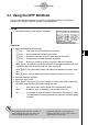
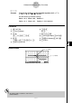
2. Select the differential equation type.
• 1(1st)........ Four types of first order differential equations
• 2(2nd) ...... Second order linear differential equations
• 3(N-th)...... Differential equations of the first order through ninth order
• 4(SYS) ..... System of the first order differential equations
• 5(RCL) ..... Displays a screen for recalling a previous differential equation.
•With 1(1st), you need to make further selections of differential equation type. See
“Differential equations of the first order” for more information.
•With 3(N-th), you also need to specify the order of the differential equation, from 1
to 9.
•With 4(SYS), you also need to specify the number of unknowns, from 1 to 9.
3. Enter the differential equation.
4. Specify the initial values.
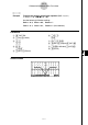
5. Press 5(SET) and select b(Param) to display the Parameter screen. Specify the
calculation range. Make the parameter settings you want.
• h................... Step size for the classical Runge-Kutta method (fourth order)
•Step ............. Number of steps for graphing*
1
and storing data in LIST.
•SF................ The number of slope field columns displayed on the screen (0 – 100).
The slope fields can be displayed only for differential equations of the
first order.
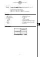
*
1
When graphed for the first time, a function is
always graphed with every step. When the
function is graphed again, however, it is
graphed according to a value of Step. For
example, when Step is set to 2, the function is
graphed with every two steps.