E ALGEBRA FX 2.0 PLUS FX 1.0 PLUS User’s Guide CASIO Worldwide Education Website http://edu.casio.com CASIO EDUCATIONAL FORUM http://edu.casio.
GUIDELINES LAID DOWN BY FCC RULES FOR USE OF THE UNIT IN THE U.S.A. (not applicable to other areas). NOTICE This equipment has been tested and found to comply with the limits for a Class B digital device, pursuant to Part 15 of the FCC Rules. These limits are designed to provide reasonable protection against harmful interference in a residential installation.
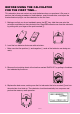
BEFORE USING THE CALCULATOR FOR THE FIRST TIME... This calculator does not contain any main batteries when you purchase it. Be sure to perform the following procedure to load batteries, reset the calculator, and adjust the contrast before trying to use the calculator for the first time. 1. Making sure that you do not accidently press the o key, slide the case onto the calculator and then turn the calculator over. Remove the back cover from the calculator by pulling with your finger at the point marked 1.
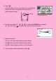
5. Press m. • If the Main Menu shown to the right is not on the display, press the P button on the back of the calculator to perform memory reset. P button * The above shows the ALGEBRA FX 2.0 PLUS screen. 6. Use the cursor keys (f, c, d, e) to select the SYSTEM icon and press ) to display the contrast adjustment screen. w, then press 2( 7. Adjust the contrast. • The e cursor key makes display contrast darker. • The d cursor key makes display contrast lighter.
Quick-Start Turning Power On And Off Using Modes Basic Calculations Replay Feature Fraction Calculations Exponents Graph Functions Dual Graph Box Zoom Dynamic Graph Table Function 19990401
1 Quick-Start Quick-Start Welcome to the world of graphing calculators. Quick-Start is not a complete tutorial, but it takes you through many of the most common functions, from turning the power on, and on to graphing complex equations. When you’re done, you’ll have mastered the basic operation of this calculator and will be ready to proceed with the rest of this user’s guide to learn the entire spectrum of functions available.
2 Quick-Start defc to highlight RUN and then press w. 2. Use • MAT This is the initial screen of the RUN • MAT Mode, where you can perform manual calculations, matrix calculations, and run programs. BASIC CALCULATIONS With manual calculations, you input formulas from left to right, just as they are written on paper. With formulas that include mixed arithmetic operators and parentheses, the calculator automatically applies true algebraic logic to calculate the result. Example: 15 × 3 + 61 1.
3 Quick-Start SET UP u3 to display the SET UP screen. 1. Press 2. Press cccc1 (Deg) to specify degrees as the angle unit. 3. Press i to clear the menu. 4. Press o to clear the unit. 5. Press cf*sefw. REPLAY FEATURE d e With the replay feature, simply press or to recall the last calculation that was performed so you can make changes or re-execute it as it is. Example: To change the calculation in the last example from (25 × sin 45˚) to (25 × sin 55˚) 1.
4 Quick-Start FRACTION CALCULATIONS $ You can use the key to input fractions into calculations. The symbol “ { ” is used to separate the various parts of a fraction. Example: 1 15/16 + 37/9 1. Press 2. Press o. b$bf$ bg+dh$ jw. Indicates 6 7/144 Converting a Mixed Fraction to an Improper Fraction d/c While a mixed fraction is shown on the display, press improper fraction. !$to convert it to an d/c Press !$again to convert back to a mixed fraction.
5 Quick-Start EXPONENTS Example: 1250 × 2.065 1. Press o. 2. Press bcfa*c.ag. 3. Press M and the ^ indicator appears on the display. 4. Press f. The ^5 on the display indicates that 5 is an exponent. 5. Press w.
6 Quick-Start GRAPH FUNCTIONS The graphing capabilities of this calculator makes it possible to draw complex graphs using either rectangular coordinates (horizontal axis: x ; vertical axis: y) or polar coordinates (angle: θ ; distance from origin: r). All of the following graphing examples are performed starting from the calculator setup in effect immediately following a reset operation. Example 1: To graph Y = X(X + 1)(X – 2) 1. Press m. defc to highlight GRPH TBL, and then press w. 2. Use • 3.
7 Quick-Start b(Root). Press e for other roots. 2. Press Example 3: Determine the area bounded by the origin and the X = –1 root obtained for Y = X(X + 1)(X – 2) 1. Press i4(G-SLV)c. 2. Press i(∫dx). d to move the pointer to the location where X = –1, and then press w. Next, use e to 3. Use move the pointer to the location where X = 0, and then press w to input the integration range, which becomes shaded on the display.
8 Quick-Start DUAL GRAPH With this function you can split the display between two areas and display two graphs on the same screen. Example: To draw the following two graphs and determine the points of intersection Y1 = X(X + 1)(X – 2) Y2 = X + 1.2 SET UP 1. Press u3ccc2(G+G) to specify “G+G” for the Dual Screen setting. i, and then input the two functions. v(v+b) (v-c)w v+b.cw 2. Press 3. Press 5(DRAW) or w to draw the graphs.
9 Quick-Start defc 3. Use to move the pointer again. As you do, a box appears on the display. Move the pointer so the box encloses the area you want to enlarge. w 4. Press , and the enlarged area appears in the inactive (right side) screen. DYNAMIC GRAPH Dynamic Graph lets you see how the shape of a graph is affected as the value assigned to one of the coefficients of its function changes. Example: To draw graphs as the value of coefficient A in the following function changes from 1 to 3 Y = AX 1.
10 Quick-Start 4 bw to assign an initial value 4. Press (VAR) of 1 to coefficient A. 5. Press 2(RANG) bwdwb wto specify the range and increment of change in coefficient A. 6. Press i. 6 7. Press (DYNA) to start Dynamic Graph drawing. The graphs are drawn 10 times.
11 Quick-Start TABLE FUNCTION The Table Function makes it possible to generate a table of solutions as different values are assigned to the variables of a function. Example: To create a number table for the following function Y = X (X+1) (X–2) 1. Press 2. Use m. defc to highlight w. GRPH • TBL, and then press 3. Input the formula. v(v+b) (v-c)w 4. Press table.
Handling Precautions • Your calculator is made up of precision components. Never try to take it apart. • Avoid dropping your calculator and subjecting it to strong impact. • Do not store the calculator or leave it in areas exposed to high temperatures or humidity, or large amounts of dust. When exposed to low temperatures, the calculator may require more time to display results and may even fail to operate. Correct operation will resume once the calculator is brought back to normal temperature.
Be sure to keep physical records of all important data! Low battery power or incorrect replacement of the batteries that power the unit can cause the data stored in memory to be corrupted or even lost entirely. Stored data can also be affected by strong electrostatic charge or strong impact. It is up to you to keep back up copies of data to protect against its loss. In no event shall CASIO Computer Co., Ltd.
• • • • • • • • • • • • • • • • • • • • • • • • • • • • • • • • • • • • • • • • • • • • • • • • • • • • • • • • • • • • • • • • • • • • • • • • • • • • • • • • • • • • • • • • • • • • • • • • • • • • • • • • • • • • • • • • • • ALGEBRA FX 2.0 PLUS FX 1.
1 Contents Contents Getting Acquainted — Read This First! Chapter 1 Basic Operation 1-1 1-2 1-3 1-4 1-5 1-6 1-7 1-8 Chapter 2 2-1 2-2 2-3 2-4 2-5 2-6 2-7 2-8 Chapter 3 3-1 3-2 3-3 3-4 Chapter 4 4-1 4-2 4-3 4-4 Keys ................................................................................................. 1-1-1 Display .............................................................................................. 1-2-1 Inputting and Editing Calculations ............................................
2 Contents Chapter 5 5-1 5-2 5-3 5-4 5-5 5-6 5-7 5-8 5-9 5-10 5-11 Chapter 6 6-1 6-2 6-3 6-4 Chapter 7 7-1 7-2 7-3 7-4 Chapter 8 8-1 8-2 8-3 8-4 8-5 8-6 8-7 8-8 Chapter 9 9-1 9-2 9-3 9-4 9-5 Graphing Sample Graphs ................................................................................ 5-1-1 Controlling What Appears on a Graph Screen ................................. 5-2-1 Drawing a Graph ..............................................................................
3 Contents Chapter 10 10-1 10-2 10-3 10-4 10-5 10-6 10-7 10-8 Data Communications Connecting Two Units .................................................................. 10-1-1 Connecting the Unit with a CASIO Label Printer .......................... 10-2-1 Connecting the Unit to a Personal Computer ............................... 10-3-1 Performing a Data Communication Operation ............................. 10-4-1 Data Communications Precautions ..............................................
4 Contents Additional Functions Chapter 1 Advanced Statistics Application 1-1 1-2 1-3 1-4 Chapter 2 2-1 2-2 2-3 2-4 2-5 2-6 2-7 2-8 2-9 2-10 2-11 Chapter 3 3-1 3-2 3-3 3-4 3-5 Chapter 4 4-1 4-2 4-3 4-4 4-5 Advanced Statistics (STAT) .............................................................. 1-1-1 Tests (TEST) .................................................................................... 1-2-1 Confidence Interval (INTR) ...............................................................
0 Getting Acquainted — Read This First! About this User’s Guide u! x( ) The above indicates you should press ! and then x, which will input a symbol. All multiple-key input operations are indicated like this. Key cap markings are shown, followed by the input character or command in parentheses. uFunction Keys and Menus • Many of the operations performed by this calculator can be executed by pressing function keys 1 through 6.
0-1-1 Getting Acquainted uGraphs As a general rule, graph operations are shown on facing pages, with actual graph examples on the right hand page. You can produce the same graph on your calculator by performing the steps under the Procedure above the graph. Look for the type of graph you want on the right hand page, and then go to the page indicated for that graph. The steps under “Procedure” always use initial RESET settings.
Chapter Basic Operation 1-1 1-2 1-3 1-4 1-5 1-6 1-7 1-8 Keys Display Inputting and Editing Calculations Option (OPTN) Menu Variable Data (VARS) Menu Program (PRGM) Menu Using the Set Up Screen When you keep having problems… 19990401 1
1-1-1 Keys 1-1 Keys COPY PASTE CAT/CAL REPLAY PRGM List H-COPY Mat i 19990401
1-1-2 Keys k Key Table Page COPY Page Page Page Page Page 1-3-5 PASTE 1-3-5 1-7-1 CAT/CAL 1-3-5 1-1-3 1-3-4 5-2-1 1-4-1 1-6-1 2-4-4 1-5-1 2-4-4 2-4-4 2-4-4 2-4-3 2-4-3 2-4-3 2-4-4 2-4-4 2-4-3 2-4-3 2-4-3 2-4-10 2-4-6 2-4-6 2-4-6 2-4-10 2-4-6 2-1-1 2-1-1 5-3-6 H-COPY 10-6-1 1-2-1 REPLAY PRGM 1-1-3 Page Page Page 2-2-1 Page Page 1-3-3 1-3-1 3-1-2 List i 2-1-1 2-1-1 2-1-1 2-1-1 2-8-11 Mat 2-4-3 2-1-1 19990401 20010102 2-2-5 2-1-1
1-1-3 Keys k Key Markings Many of the calculator’s keys are used to perform more than one function. The functions marked on the keyboard are color coded to help you find the one you need quickly and easily. Function Key Operation l 1 log 2 x 10 !l 3 B al The following describes the color coding used for key markings. Color # Key Operation Orange Press ! and then the key to perform the marked function. Red Press a and then the key to perform the marked function.
1-2-1 Display 1-2 Display k Selecting Icons This section describes how to select an icon in the Main Menu to enter the mode you want. uTo select an icon 1. Press m to display the Main Menu. 2. Use the cursor keys (d, e, f, c) to move the highlighting to the icon you want. Currently selected icon * The above shows the ALGEBRA FX 2.0 PLUS screen. 3. Press w to display the initial screen of the mode whose icon you selected. Here we will enter the STAT Mode.
1-2-2 Display Icon Mode Name Description GRaPH-TaBLe Use this mode to store functions, to generate a numeric table of different solutions as the values assigned to variables in a function change, and to draw graphs. DYNAmic graph Use this mode to store graph functions and to draw multiple versions of a graph by changing the values assigned to the variables in a function.
1-2-3 Display k About the Function Menu Use the function keys (1 to 6) to access the menus and commands in the menu bar along the bottom of the display screen. You can tell whether a menu bar item is a menu or a command by its appearance. • Command (Example: ) Pressing a function key that corresponds to a menu bar command executes the command. • Pull-up Menu (Example: ) Pressing a function key that corresponds to a pull-up menu opens the menu.
1-2-4 Display k Normal Display The calculator normally displays values up to 10 digits long. Values that exceed this limit are automatically converted to and displayed in exponential format. u How to interpret exponential format 1.2E+12 indicates that the result is equivalent to 1.2 × 10¹². This means that you should move the decimal point in 1.2 twelve places to the right, because the exponent is positive. This results in the value 1,200,000,000,000. 1.
1-2-5 Display k Special Display Formats This calculator uses special display formats to indicate fractions, hexadecimal values, and degrees/minutes/seconds values. u Fractions 12 ................. Indicates: 456 –––– 23 u Hexadecimal Values ................. Indicates: ABCDEF12(16), which equals –1412567278(10) u Degrees/Minutes/Seconds ................. Indicates: 12° 34’ 56.
1-3-1 Inputting and Editing Calculations 1-3 Inputting and Editing Calculations k Inputting Calculations When you are ready to input a calculation, first press A to clear the display. Next, input your calculation formulas exactly as they are written, from left to right, and press w to obtain the result.
1-3-2 Inputting and Editing Calculations u To delete a step ○ ○ ○ ○ ○ Example To change 369 × × 2 to 369 × 2 Adgj**c ddD u To insert a step ○ ○ ○ ○ ○ Example To change 2.362 to sin2.362 Ac.
1-3-3 Inputting and Editing Calculations k Using Replay Memory The last calculation performed is always stored into replay memory. You can recall the contents of the replay memory by pressing d or e. If you press e, the calculation appears with the cursor at the beginning. Pressing d causes the calculation to appear with the cursor at the end. You can make changes in the calculation as you wish and then execute it again. ○ ○ ○ ○ ○ Example 1 To perform the following two calculations 4.12 × 6.4 = 26.368 4.
1-3-4 Inputting and Editing Calculations k Making Corrections in the Original Calculation ○ ○ ○ ○ ○ Example 14 ÷ 0 × 2.3 entered by mistake for 14 ÷ 10 × 2.3 Abe/a*c.d w Press i. Cursor is positioned automatically at the location of the cause of the error. Make necessary changes. db Execute again. w k Copy and Paste You can temporarily copy commands, programs, and other text data you input to a memory area called “the clipboard,” and then paste it to another location on the display.
1-3-5 Inputting and Editing Calculations 3. Press u1 (COPY) to copy the highlighted text to the clipboard, and exit the copy range specification mode. To cancel text highlighting without performing a copy operation, press i. u Pasting Text Move the cursor to the location where you want to paste the text, and then press u 2(PASTE). The contents of the clipboard are pasted at the cursor position.
1-3-6 Inputting and Editing Calculations ○ ○ ○ ○ ○ Example 2 To use the Catalog to input the Prog command Au4(CAT/CAL)6(g)6(g) 5(P)I(Prog) Pressing i or !i(QUIT) closes the Catalog.
1-4-1 Option (OPTN) Menu 1-4 Option (OPTN) Menu The option menu gives you access to scientific functions and features that are not marked on the calculator’s keyboard. The contents of the option menu differ according to the mode you are in when you press the K key. See “8-7 Program Mode Command List” for details on the option (OPTN) menu. u Option Menu in the RUN • MAT or PRGM Mode • {LIST} ... {list function menu} • {MAT} ... {matrix operation menu} • {CPLX} ...
1-4-2 Option (OPTN) Menu The following shows the function menus that appear under other conditions. u Option Menu when a number table value is displayed in the GRPH • TBL or RECUR Mode • {LMEM} … {list memory menu} •{ ° ’ ”}/{ENG}/{ ENG} u Option Menu in the CAS or ALGEBRA or TUTOR Mode (ALGEBRA FX 2.
1-5-1 Variable Data (VARS) Menu 1-5 Variable Data (VARS) Menu To recall variable data, press J to display the variable data menu. {V-WIN}/{FACT}/{STAT}/{GRPH}/{DYNA}/ {TABL}/{RECR}/{EQUA*1} See “8-7 Program Mode Command List” for details on the variable data (VARS) menu.
1-5-2 Variable Data (VARS) Menu u STAT — Recalling statistical data • {n} … {number of data} • {X} … {single-variable, paired-variable x-data} • {o }/{Σ x }/{Σ x 2 }/{x σn }/{x σ n –1 }/{minX}/{maxX} …{mean}/{sum}/{sum of squares}/{population standard deviation}/{sample standard deviation}/{minimum value}/{maximum value} • {Y} ...
1-5-3 Variable Data (VARS) Menu u GRPH — Recalling Graph Functions • {Yn }/{rn } ... {rectangular coordinate or inequality function}/{polar coordinate function} • {Xtn }/{Yt n } ... parametric graph function {Xt}/{Yt} • {Xn } ... {X=constant graph function} (Press these keys before inputting a value to specify a storage area.) u DYNA — Recalling Dynamic Graph Set Up Data • {Start}/{End}/{Pitch} ...
1-5-4 Variable Data (VARS) Menu u RECR — Recalling Recursion Formula*1, Table Range, and Table Content Data • {FORM} ... {recursion formula data menu} • {an}/{an+1}/{an+2}/{bn}/{bn+1}/{bn+2}/{cn}/{cn+1}/{cn+2} ... {an}/{an+1}/{an+2}/{bn}/{bn+1}/{bn+2}/{cn}/{cn+1}/{cn+2} expressions • {RANGE} ... {table range data menu} • {R-Strt}/{R-End} ... table range {start value}/{end value} • {a0}/{a1}/{a2}/{b0}/{b1}/{b2}/{c0}/{c1}/{c2} ...
1-6-1 Program (PRGM) Menu 1-6 Program (PRGM) Menu To display the program (PRGM) menu, first enter the RUN • MAT or PRGM Mode from the Main Menu and then press !J(PRGM). The following are the selections available in the program (PRGM) menu. • {Prog } ........ {program recall} • {JUMP} ...... {jump command menu} • {? } .............. {input prompt} • {^} ............. {output command} • {I/O} ............ {I/O control/transfer command menu} • {IF } ............. {conditional jump command menu} • {FOR} ......
1-7-1 Using the Set Up Screen 1-7 Using the Set Up Screen The mode’s set up screen shows the current status of mode settings and lets you make any changes you want. The following procedure shows how to change a set up. u To change a mode set up 1. Select the icon you want and press w to enter a mode and display its initial screen. Here we will enter the RUN • MAT Mode. 2. Press u3(SET UP) to display the mode’s SET UP screen. ... • This SET UP screen is just one possible example.
1-7-2 Using the Set Up Screen u Func Type (graph function type) Pressing one of the following function keys also switches the function of the v key. • {Y=}/{r=}/{Parm}/{X=c} ... {rectangular coordinate}/{polar coordinate}/{parametric coordinate}/ {X = constant} graph • {Y>}/{Y<}/{Yt}/{Ys} ... {y>f(x)}/{y
1-7-3 Using the Set Up Screen u Display (display format) • {Fix}/{Sci}/{Norm}/{Eng} ... {fixed number of decimal places specification}/{number of significant digits specification}/{normal display setting}/{Engineering Mode} u Stat Wind (statistical graph view window setting method) • {Auto}/{Man} ... {automatic}/{manual} u Reside List (residual calculation) • {None}/{LIST} ... {no calculation}/{list specification for the calculated residual data} u List File (list file display settings) • {FILE} ...
1-7-4 Using the Set Up Screen u Dynamic Type (Dynamic Graph locus setting) • {Cnt}/{Stop} ... {non-stop (continuous)}/{automatic stop after 10 draws} u Σ Display (Σ value display in recursion table) • {On}/{Off} ... {display on}/{display off} u Slope (display of derivative at current pointer location in conic section graph) • {On}/{Off} ... {display on}/{display off} u Answer Type (result range specification) (ALGEBRA FX 2.0 PLUS only) • {Real}/{Cplx} ...
1-8-1 When you keep having problems… 1-8 When you keep having problems… If you keep having problems when you are trying to perform operations, try the following before assuming that there is something wrong with the calculator. k Getting the Calculator Back to its Original Mode Settings 1. From the Main Menu, enter the SYSTEM Mode. 2. Press 5(Reset). 3. Press 1(S/U), and then press w(Yes). 4. Press m to return to the Main Menu.
1-8-2 When you keep having problems… k Low Battery Message If either of the following messages appears on the display, immediately turn off the calculator and replace main batteries or the back up battery as instructed. If you continue using the calculator without replacing main batteries, power will automatically turn off to protect memory contents. Once this happens, you will not be able to turn power back on, and there is the danger that memory contents will be corrupted or lost entirely.
Chapter Manual Calculations 2-1 2-2 2-3 2-4 2-5 2-6 2-7 2-8 Basic Calculations Special Functions Specifying the Angle Unit and Display Format Function Calculations Numerical Calculations Complex Number Calculations Binary, Octal, Decimal, and Hexadecimal Calculations Matrix Calculations 20010101 2
2-1-1 Basic Calculations 2-1 Basic Calculations k Arithmetic Calculations • Enter arithmetic calculations as they are written, from left to right. • Use the - key to input the minus sign before a negative value. • Calculations are performed internally with a 15-digit mantissa. The result is rounded to a 10-digit mantissa before it is displayed. • For mixed arithmetic calculations, multiplication and division are given priority over addition and subtraction. Example Operation 23 + 4.5 – 53 = –25.5 23+4.
2-1-2 Basic Calculations k Number of Decimal Places, Number of Significant Digits, Normal Display Range [SET UP]- [Display] -[Fix] / [Sci] / [Norm] • Even after you specify the number of decimal places or the number of significant digits, internal calculations are still performed using a 15-digit mantissa, and displayed values are stored with a 10-digit mantissa.
2-1-3 Basic Calculations ○ ○ ○ ○ ○ Example 200 ÷ 7 × 14 = 400 Condition 3 decimal places Operation Display 200/7*14w u3(SET UP)cccccccccc 1(Fix)dwiw Calculation continues using display capacity of 10 digits 200/7w * 14w 400 400.000 28.571 Ans × 400.000 • If the same calculation is performed using the specified number of digits: 200/7w The value stored internally is rounded off to the number of decimal places you specify. K5(NUM)e(Rnd)w * 14w 28.571 28.571 Ans × 399.
2-1-4 Basic Calculations 3 Power/root ^(xy), x 4 Fractions a b/c 5 Abbreviated multiplication format in front of π, memory name, or variable name. 2π, 5A, Xmin, F Start, etc. 6 Type B functions With these functions, the function key is pressed and then the value is entered.
2-1-5 Basic Calculations k Multiplication Operations without a Multiplication Sign You can omit the multiplication sign (×) in any of the following operations. • Before coordinate transformation and Type B functions (1 on page 2-1-3 and 6 on page 2-1-4), except for negative signs ○ ○ ○ ○ ○ Example 2sin30, 10log1.2, 2 , 2Pol(5, 12), etc. • Before constants, variable names, memory names ○ ○ ○ ○ ○ Example 2π, 2AB, 3Ans, 3Y1, etc.
2-1-6 Basic Calculations • When you try to perform a calculation that causes memory capacity to be exceeded (Memory ERROR). • When you use a command that requires an argument, without providing a valid argument (Argument ERROR). • When an attempt is made to use an illegal dimension during matrix calculations (Dimension ERROR). • When you are in the real mode and an attempt is made to perform a calculation that produces a complex number solution.
2-2-1 Special Functions 2-2 Special Functions k Calculations Using Variables Example Operation Display 193.2aav(A)w 193.2 193.2 ÷ 23 = 8.4 av(A)/23w 8.4 193.2 ÷ 28 = 6.9 av(A)/28w 6.9 k Memory u Variables This calculator comes with 28 variables as standard. You can use variables to store values you want to use inside of calculations. Variables are identified by single-letter names, which are made up of the 26 letters of the alphabet, plus r and θ.
2-2-2 Special Functions u To display the contents of a variable ○ ○ ○ ○ ○ Example To display the contents of variable A Aav(A)w u To clear a variable ○ ○ ○ ○ ○ Example To clear variable A Aaaav(A)w u To assign the same value to more than one variable [value]a [first variable name*1]K6(g)6(g)4(SYBL)d(~) [last variable name*1]w ○ ○ ○ ○ ○ Example To assign a value of 10 to variables A through F Abaaav(A) K6(g)6(g)4(SYBL)d(~) at(F)w u Function Memory [OPTN]-[FMEM] Function memory (f1~f20) is conveni
2-2-3 Special Functions u To store a function ○ ○ ○ ○ ○ Example To store the function (A+B) (A–B) as function memory number 1 (av(A)+al(B)) (av(A)-al(B)) K6(g)5(FMEM) b(Store)bw u To recall a function ○ ○ ○ ○ ○ Example To recall the contents of function memory number 1 K6(g)5(FMEM) c(Recall)bw u To display a list of available functions K6(g)5(FMEM) e(SEE) # If the function memory number to which you store a function already contains a function, the previous function is replaced with the new one.
2-2-4 Special Functions u To delete a function ○ ○ ○ ○ ○ Example To delete the contents of function memory number 1 AK6(g)5(FMEM) b(Store)bw • Executing the store operation while the display is blank deletes the function in the function memory you specify. u To use stored functions ○ ○ ○ ○ ○ Example To store x3 + 1, x2 + x into function memory, and then graph: y = x3 + x2 + x + 1 Use the following View Window settings.
2-2-5 Special Functions k Answer Function The Answer Function automatically stores the last result you calculated by pressing w(unless the w key operation results in an error). The result is stored in the answer memory. u To use the contents of the answer memory in a calculation ○ ○ ○ ○ ○ Example 123 + 456 = 579 789 – 579 = 210 Abcd+efgw hij-!-(Ans)w k Performing Continuous Calculations Answer memory also lets you use the result of one calculation as one of the arguments in the next calculation.
2-2-6 Special Functions k Stacks The unit employs memory blocks, called stacks, for storage of low priority values and commands. There is a 10-level numeric value stack, a 26-level command stack, and a 10level program subroutine stack. An error occurs if you perform a calculation so complex that it exceeds the capacity of available numeric value stack or command stack space, or if execution of a program subroutine exceeds the capacity of the subroutine stack.
2-2-7 Special Functions k Using Multistatements Multistatements are formed by connecting a number of individual statements for sequential execution. You can use multistatements in manual calculations and in programmed calculations. There are two different ways that you can use to connect statements to form multistatements. • Colon (:) Statements that are connected with colons are executed from left to right, without stopping.
2-3-1 Specifying the Angle Unit and Display Format 2-3 Specifying the Angle Unit and Display Format Before performing a calculation for the first time, you should use the SET UP screen to specify the angle unit and display format. k Setting the Angle Unit [SET UP]- [Angle] 1. On the Set Up screen, highlight “Angle”. 2. Press the function key for the angle unit you want to specify, then press i. • {Deg}/{Rad}/{Gra} ...
2-3-2 Specifying the Angle Unit and Display Format u To specify the number of significant digits (Sci) ○ ○ ○ ○ ○ Example To specify three significant digits 2(Sci) dw Press the function key that corresponds to the number of significant digits you want to specify (n = 0 to 9). u To specify the normal display (Norm 1/Norm 2) Press 3(Norm) to switch between Norm 1 and Norm 2. Norm 1: 10–2 (0.01)>|x|, |x| >1010 Norm 2: 10–9 (0.
2-4-1 Function Calculations 2-4 Function Calculations k Function Menus This calculator includes five function menus that give you access to scientific functions not printed on the key panel. • The contents of the function menu differ according to the mode you entered from the Main Menu before you pressed the K key. The following examples show function menus that appear in the RUN • MAT Mode. u Numeric Calculations (NUM) [OPTN]-[NUM] • {Abs} ...
2-4-2 Function Calculations u Hyperbolic Calculations (HYP) [OPTN]-[HYP] • {sinh}/{cosh}/{tanh} ... hyperbolic {sine}/{cosine}/{tangent} • {sinh–1}/{cosh–1}/{tanh–1} ... inverse hyperbolic {sine}/{cosine}/{tangent} u Angle Units, Coordinate Conversion, Sexagesimal Operations (ANGL) [OPTN]-[ANGL] • {°}/{r}/{g} ... {degrees}/{radians}/{grads} for a specific input value • {° ’ ”} ... {specifies degrees (hours), minutes, seconds when inputting a degrees/minutes/ seconds value} • {'DMS} ...
2-4-3 Function Calculations k Trigonometric and Inverse Trigonometric Functions • Be sure to set the angle unit before performing trigonometric function and inverse trigonometric function calculations. π (90° = ––– radians = 100 grads) 2 • Be sure to specify Comp for Mode in the SET UP screen. Example sin 63° = 0.8910065242 π cos (–– rad) = 0.5 3 Operation u3(SET UP)cccc1(Deg)i s63w u3(SET UP)cccc2(Rad)i c(!E(π)/d)w tan (– 35gra) = – 0.6128007881 u3(SET UP)cccc3(Gra)i t-35w 2 • sin 45° × cos 65° = 0.
2-4-4 Function Calculations k Logarithmic and Exponential Functions • Be sure to specify Comp for Mode in the SET UP screen. Example Operation log 1.23 (log101.23) = 8.990511144 × 10⁻² l1.23w In 90 (loge90) = 4.49980967 I90w 101.23 = 16.98243652 (To obtain the antilogarithm of common logarithm 1.23) !l(10x)1.23w e4.5 = 90.0171313 (To obtain the antilogarithm of natural logarithm 4.5) !I(ex)4.
2-4-5 Function Calculations k Hyperbolic and Inverse Hyperbolic Functions • Be sure to specify Comp for Mode in the SET UP screen. Example Operation sinh 3.6 = 18.28545536 K6(g)2(HYP)b(sinh)3.6w cosh 1.5 – sinh 1.5 = 0.2231301601 = e –1.5 (Display: –1.5) K6(g)2(HYP)c(cosh)1.52(HYP)b(sinh)1.5w I!-(Ans)w (Proof of cosh x ± sinh x = e±x) cosh–1 20 15 = 0.7953654612 K6(g)2(HYP)f(cosh–1)(20/15)w Determine the value of x when tanh 4 x = 0.88 –1 x = tanh 0.88 K6(g)2(HYP)g(tanh–1)0.88/4w 4 = 0.
2-4-6 Function Calculations k Other Functions • Be sure to specify Comp for Mode in the SET UP screen. Example Operation 2 + 5 = 3.65028154 !x( )2+!x( (3 + i) = 1.755317302 +0.2848487846i !x( )(d+!a(i))w (–3)2 = (–3) × (–3) = 9 (-3)xw –32 = –(3 × 3) = –9 -3xw 1 –––––– = 12 1 1 –– – –– 3 4 8! (= 1 × 2 × 3 × .... × 8) = 40320 3 36 × 42 × 49 = 42 What is the absolute value of 3 the common logarithm of ? 4 | log 34 | = 0.
2-4-7 Function Calculations k Random Number Generation (Ran#) This function generates a 10-digit truly random or sequentially random number that is greater than zero and less than 1. • A truly random number is generated if you do not specify anything for the argument. Example Operation Ran # (Generates a random number.) K6(g)1(PROB)e(Ran#)w (Each press of w generates a new random number.) w w • Specifying an argument from 1 to 9 generates random numbers based on that sequence.
2-4-8 Function Calculations k Coordinate Conversion u Rectangular Coordinates u Polar Coordinates • With polar coordinates, θ can be calculated and displayed within a range of –180°< θ < 180° (radians and grads have same range). • Be sure to specify Comp for Mode in the SET UP screen. Example Operation Calculate r and θ ° when x = 14 and y = 20.7 1 24.989 → 24.98979792 (r) 2 55.928 → 55.92839019 (θ) u3(SET UP)cccc1(Deg)i K6(g)3(ANGL)g(Pol() 14,20.7)w Calculate x and y when r = 25 and θ = 56° 1 13.
2-4-9 Function Calculations k Permutation and Combination u Permutation u Combination n! nPr = ––––– (n – r)! n! nCr = ––––––– r! (n – r)! • Be sure to specify Comp for Mode in the SET UP screen.
2-4-10 Function Calculations k Fractions • Fractional values are displayed with the integer first, followed by the numerator and then the denominator. • Be sure to specify Comp for Mode in the SET UP screen. Example Operation 2 1 13 –– + 3 –– = 3 ––– (Display: 3{13{20) 5 4 20 = 3.65 1 1 ––––– + ––––– = 6.066202547 × 10⁻⁴ 2578 4572 2$5+3$1$4w $(Conversion to decimal) $(Conversion to fraction) 1$2578+1$4572w (Display: 6.066202547E–04*1 ) (Norm 1 display format) 1 –– × 0.5 = 0.25*2 2 1 = –– 4 1$2*.
2-4-11 Function Calculations k Engineering Notation Calculations Input engineering symbols using the engineering notation menu. • Be sure to specify Comp for Mode in the SET UP screen. Example Operation 999k (kilo) + 25k (kilo) = 1.024M (mega) u3(SET UP)cccccccccc 4(Eng)i 999K5(NUM)g(E-SYM)g(k)+255(NUM) g(E-SYM)g(k)w 9 ÷ 10 = 0.9 = 900m (milli) = 0.9 = 0.0009k (kilo) = 0.
2-5-1 Numerical Calculations 2-5 Numerical Calculations The following describes the items that are available in the menus you use when performing differential/ quadratic differential, integration, Σ, maximum/minimum value, and Solve calculations. When the option menu is on the display, press 4(CALC) to display the function analysis menu. The items of this menu are used when performing specific types of calculations. • {d/dx}/{d2/dx2}/{∫dx}/{Σ}/{FMin}/{FMax}/{Solve} ...
2-5-2 Numerical Calculations k Differential Calculations [OPTN]-[CALC]-[d /dx] To perform differential calculations, first display the function analysis menu, and then input the values shown in the formula below.
2-5-3 Numerical Calculations ○ ○ ○ ○ ○ Example To determine the derivative at point x = 3 for the function y = x3 + 4 x2 + x – 6, with a tolerance of “tol” = 1E – 5 Input the function f(x). AK4(CALC)b(d/dx)vMd+evx+v-g, Input point x = a for which you want to determine the derivative. d, Input the tolerance value. bE-f) w # In the function f(x), only X can be used as a variable in expressions.
2-5-4 Numerical Calculations u Applications of Differential Calculations • Differentials can be added, subtracted, multiplied or divided with each other. d d ––– f (a) = f '(a), ––– g (a) = g'(a) dx dx Therefore: f '(a) + g'(a), f '(a) × g'(a), etc. • Differential results can be used in addition, subtraction, multiplication, and division, and in functions. 2 × f '(a), log ( f '(a)), etc. • Functions can be used in any of the terms ( f (x), a, tol) of a differential. d ––– (sinx + cosx, sin0.
2-5-5 Numerical Calculations k Quadratic Differential Calculations [OPTN]-[CALC]-[d 2 /dx2] After displaying the function analysis menu, you can input quadratic differentials using either of the two following formats.
2-5-6 Numerical Calculations u Quadratic Differential Applications • Arithmetic operations can be performed using two quadratic differentials. d2 d2 –––2 f (a) = f ''(a), ––– g (a) = g''(a) dx dx 2 Therefore: f ''(a) + g''(a), f ''(a) × g''(a), etc. • The result of a quadratic differential calculation can be used in a subsequent arithmetic or function calculation. 2 × f ''(a), log ( f ''(a) ), etc. • Functions can be used within the terms ( f(x), a, tol ) of a quadratic differential expression.
2-5-7 Numerical Calculations k Integration Calculations [OPTN]-[CALC]-[∫dx] To perform integration calculations, first display the function analysis menu and then input the values in the formula shown below.
2-5-8 Numerical Calculations ○ ○ ○ ○ ○ Example To perform the integration calculation for the function shown below, with a tolerance of “tol” = 1E - 4 ∫ 5 1 (2x2 + 3x + 4) dx Input the function f (x). AK4(CALC)d(∫dx)cvx+dv+e, Input the start point and end point. b,f, Input the tolerance value. bE-e) w u Application of Integration Calculation • Integrals can be used in addition, subtraction, multiplication or division. ∫ b a f(x) dx + ∫ d c g (x) dx, etc.
2-5-9 Numerical Calculations Note the following points to ensure correct integration values. (1) When cyclical functions for integration values become positive or negative for different divisions, perform the calculation for single cycles, or divide between negative and positive, and then add the results together.
2-5-10 Numerical Calculations k Σ Calculations [OPTN]-[CALC]-[Σ ] To perform Σ calculations, first display the function analysis menu, and then input the values shown in the formula below. K4(CALC)e(Σ) a k , k , α , β , n ) β Σ (a , k, α, β, n) = Σ a = a k α k k=α + aα +1 +........+ aβ (n: distance between partitions) ○ ○ ○ ○ ○ Example To calculate the following: 6 Σ (k 2 – 3k + 5) k=2 Use n = 1 as the distance between partitions.
2-5-11 Numerical Calculations u Σ Calculation Applications • Arithmetic operations using Σ calculation expressions n n k=1 k=1 Sn = Σ ak, Tn = Σ bk Expressions: Sn + Tn, Sn – Tn, etc. Possible operations: • Arithmetic and function operations using Σ calculation results 2 × Sn, log (Sn), etc. • Function operations using Σ calculation terms (ak, k) Σ (sink, k, 1, 5), etc.
2-5-12 Numerical Calculations k Maximum/Minimum Value Calculations [OPTN]-[CALC]-[FMin]/[FMax] After displaying the function analysis menu, you can input maximum/minimum calculations using the formats below, and solve for the maximum and minimum of a function within interval a < x < b.
2-5-13 Numerical Calculations ○ ○ ○ ○ ○ Example 2 To determine the maximum value for the interval defined by start point a = 0 and end point b = 3, with a precision of n = 6 for the function y = –x2 + 2 x + 2 Input f(x). AK4(CALC)g(FMax) -vx+cv+c, Input the interval a = 0, b = 3. a,d, Input the precision n = 6. g) w # In the function f(x), only X can be used as a variable in expressions.
2-6-1 Complex Number Calculations 2-6 Complex Number Calculations You can perform addition, subtraction, multiplication, division, parentheses calculations, function calculations, and memory calculations with complex numbers just as you do with the manual calculations described on pages 2-1-1 and 2-4-6. You can select the complex number calculation mode by changing the Complex Mode item on the SET UP screen to one of the following settings. • {Real} ...
2-6-2 Complex Number Calculations k Absolute Value and Argument [OPTN]-[CPLX]-[Abs]/[Arg] The unit regards a complex number in the form a + bi as a coordinate on a Gaussian plane, and calculates absolute value Z and argument (arg).
2-6-3 Complex Number Calculations k Conjugate Complex Numbers [OPTN]-[CPLX]-[Conjg] A complex number of the form a + bi becomes a conjugate complex number of the form a – bi. ○ ○ ○ ○ ○ Example To calculate the conjugate complex number for the complex number 2 + 4i AK3(CPLX)d(Conjg) (c+e!a(i))w k Extraction of Real and Imaginary Parts [OPTN]-[CPLX]-[ReP]/[lmP] Use the following procedure to extract the real part a and the imaginary part b from a complex number of the form a + bi.
2-6-4 Complex Number Calculations k Polar Form and Rectangular Transformation [OPTN]-[CPLX]-[ ' re ^ θ i] Use the following procedure to transform a complex number displayed in rectangular form to polar form, and vice versa.
2-7-1 Binary, Octal, Decimal, and Hexadecimal Calculations with Integers 2-7 Binary, Octal, Decimal, and Hexadecimal Calculations with Integers You can use the RUN • MAT Mode and binary, octal, decimal, and hexadecimal settings to perform calculations that involve binary, octal, decimal and hexadecimal values. You can also convert between number systems and perform bitwise operations. • You cannot use scientific functions in binary, octal, decimal, and hexadecimal calculations.
2-7-2 Binary, Octal, Decimal, and Hexadecimal Calculations with Integers • The following are the calculation ranges for each of the number systems.
2-7-3 Binary, Octal, Decimal, and Hexadecimal Calculations with Integers k Selecting a Number System You can specify decimal, hexadecimal, binary, or octal as the default number system using the set up screen. After you press the function key that corresponds to the system you want to use, press w. u To specify a number system for an input value You can specify a number system for each individual value you input. Press 1(d~o) to display a menu of number system symbols.
2-7-4 Binary, Octal, Decimal, and Hexadecimal Calculations with Integers ○ ○ ○ ○ ○ Example 2 To input and execute 1238 × ABC16, when the default number system is decimal or hexadecimal u3(SET UP)2(Dec)i A1(d~o)e(o)bcd* 1(d~o)c(h)ABC*1w 3(DISP)c(Hex)w k Negative Values and Bitwise Operations Press 2(LOGIC) to display a menu of negation and bitwise operators. • {Neg} ... {negation}*2 • {Not}/{and}/{or}/{xor}/{xnor} ...
2-7-5 Binary, Octal, Decimal, and Hexadecimal Calculations with Integers ○ ○ ○ ○ ○ Example 2 To display the result of “368 or 11102” as an octal value u3(SET UP)5(Oct)i Adg2(LOGIC) e(or)1(d~o)d(b) bbbaw ○ ○ ○ ○ ○ Example 3 To negate 2FFFED16 u3(SET UP)3(Hex)i A2(LOGIC)c(Not) cFFFED*1w u Number System Transformation Press 3(DISP) to display a menu of number system transformation functions. • {'Dec}/{'Hex}/{'Bin}/{'Oct} ...
2-8-1 Matrix Calculations 2-8 Matrix Calculations From the Main Menu, enter the RUN • MAT Mode, and press 1(MAT) to perform Matrix calculations. 26 matrix memories (Mat A through Mat Z) plus a Matrix Answer Memory (MatAns), make it possible to perform the following matrix operations.
2-8-2 Matrix Calculations k Inputting and Editing Matrices Pressing 1(MAT) displays the matrix editor screen. Use the matrix editor to input and edit matrices. m × n … m (row) × n (column) matrix None… no matrix preset • {DIM} ... {specifies the matrix dimensions (number of cells)} • {DEL}/{DEL·A} ... deletes {a specific matrix}/{all matrices} u Creating a Matrix To create a matrix, you must first define its dimensions (size) in the Matrix list. Then you can input values into the matrix.
2-8-3 Matrix Calculations u To input cell values ○ ○ ○ ○ ○ Example To input the following data into Matrix B : 1 2 3 4 5 6 c (Selects Mat B.) w bwcwdw ewfwgw (Data is input into the highlighted cell. Each time you press w, the highlighting moves to the next cell to the right.) # You can input complex numbers into the cell of a matrix. # Displayed cell values show positive integers up to six digits, and negative integers up to five digits (one digit used for the negative sign).
2-8-4 Matrix Calculations u Deleting Matrices You can delete either a specific matrix or all matrices in memory. u To delete a specific matrix 1. While the Matrix list is on the display, use f and c to highlight the matrix you want to delete. 2. Press 2(DEL). 3. Press w(Yes) to delete the matrix or i(No) to abort the operation without deleting anything. u To delete all matrices 1. While the Matrix list is on the display, press 3(DEL·A). 2.
2-8-5 Matrix Calculations k Matrix Cell Operations Use the following procedure to prepare a matrix for cell operations. 1. While the Matrix list is on the display, use f and c to highlight the name of the matrix you want to use. You can jump to a specific matrix by inputting the letter that corresponds to the matrix name. Inputting ai(N), for example, jumps to Mat N. Pressing !-(Ans) jumps to the Matrix current Memory. 2. Press w and the function menu with the following items appears. • {EDIT} ...
2-8-6 Matrix Calculations u To calculate the scalar multiplication of a row ○ ○ ○ ○ ○ Example To calculate the product of row 2 of the following matrix and the scalar 4: Matrix A = 1 2 3 4 5 6 2(R-OP)c(×Row) Input multiplier value. ew Specify row number.
2-8-7 Matrix Calculations u To add two rows together ○ ○ ○ ○ ○ Example To add row 2 to row 3 of the following matrix : Matrix A = 1 2 3 4 5 6 2(R-OP)e(Row+) Specify number of row to be added. cw Specify number of row to be added to. dw 6(EXE) (orw) u Row Operations • {R • DEL} ... {delete row} • {R • INS} ... {insert row} • {R • ADD} ...
2-8-8 Matrix Calculations u To insert a row ○ ○ ○ ○ ○ Example To insert a new row between rows one and two of the following matrix : Matrix A = 1 2 3 4 5 6 c 4(R • INS) u To add a row ○ ○ ○ ○ ○ Example To add a new row below row 3 of the following matrix : Matrix A = 1 2 3 4 5 6 cc 5(R • ADD) 20010101
2-8-9 Matrix Calculations u Column Operations • {C • DEL} ... {delete column} • {C • INS} ... {insert column} • {C • ADD} ...
2-8-10 Matrix Calculations u To add a column ○ ○ ○ ○ ○ Example To add a new column to the right of column 2 of the following matrix : Matrix A = 1 2 3 4 5 6 e 6(g)3(C • ADD) k Modifying Matrices Using Matrix Commands [OPTN]-[MAT] u To display the matrix commands 1. From the Main Menu, enter the RUN • MAT Mode. 2. Press K to display the option menu. 3. Press 2(MAT) to display the matrix command menu.
2-8-11 Matrix Calculations u Matrix Data Input Format [OPTN]-[MAT]-[Mat] The following shows the format you should use when inputting data to create a matrix using the Mat command. a11 a12 a21 a22 a1n a2n am1 am2 amn = [ [a11, a12, ..., a1n] [a21, a22, ..., a2n] .... [am1, am2, ...
2-8-12 Matrix Calculations u To input an identity matrix [OPTN]-[MAT]-[Ident] Use the Identity command to create an identity matrix. ○ ○ ○ ○ ○ Example 2 To create a 3 × 3 identity matrix as Matrix A K2(MAT)g(Ident) da2(MAT)b(Mat)av(A)w Number of rows/columns u To check the dimensions of a matrix [OPTN]-[MAT]-[Dim] Use the Dim command to check the dimensions of an existing matrix.
2-8-13 Matrix Calculations u Modifying Matrices Using Matrix Commands You can also use matrix commands to assign values to and recall values from an existing matrix, to fill in all cells of an existing matrix with the same value, to combine two matrices into a single matrix, and to assign the contents of a matrix column to a list file.
2-8-14 Matrix Calculations u To fill a matrix with identical values and to combine two matrices into a single matrix [OPTN]-[MAT]-[Fill]/[Augmnt] Use the Fill command to fill all the cells of an existing matrix with an identical value and the Augment command to combine two existing matrices into a single matrix.
2-8-15 Matrix Calculations u To assign the contents of a matrix column to a list [OPTN]-[MAT]-[M→List] Use the following format with the Mat→List command to specify a column and a list.
2-8-16 Matrix Calculations k Matrix Calculations [OPTN]-[MAT] Use the matrix command menu to perform matrix calculation operations. u To display the matrix commands 1. From the Main Menu, enter the RUN • MAT Mode. 2. Press K to display the option menu. 3. Press 2(MAT) to display the matrix command menu. The following describes only the matrix commands that are used for matrix arithmetic operations. • {Mat} ... {Mat command (matrix specification)} • {Det} ... {Det command (determinant command)} • {Trn} .
2-8-17 Matrix Calculations u Matrix Arithmetic Operations [OPTN]-[MAT]-[Mat] ○ ○ ○ ○ ○ Example 1 To add the following two matrices (Matrix A + Matrix B) : A= 1 1 2 1 B= 2 3 2 1 AK2(MAT)b(Mat)av(A)+ 2(MAT)b(Mat)al(B)w ○ ○ ○ ○ ○ Example 2 Calculate the product to the following matrix using a multiplier value of 5 : Matrix A = 1 2 3 4 AfK2(MAT)b(Mat) av(A)w ○ ○ ○ ○ ○ Example 3 To multiply the two matrices in Example 1 (Matrix A × Matrix B) AK2(MAT)b(Mat)av(A)* 2(MAT)b(Mat)al(B)w ○ ○ ○
2-8-18 Matrix Calculations u Determinant [OPTN]-[MAT]-[Det] ○ ○ ○ ○ ○ Example Obtain the determinant for the following matrix : 1 2 3 4 5 6 –1 –2 0 Matrix A = K2(MAT)d(Det)2(MAT)b(Mat) av(A)w u Matrix Transposition [OPTN]-[MAT]-[Trn] A matrix is transposed when its rows become columns and its columns become rows.
2-8-19 Matrix Calculations u Matrix Inversion [OPTN]-[MAT]-[x –1] ○ ○ ○ ○ ○ Example To invert the following matrix : Matrix A = 1 2 3 4 K2(MAT)b(Mat) av(A)!) (x–1) w u Squaring a Matrix [OPTN]-[MAT]-[x 2] ○ ○ ○ ○ ○ Example To square the following matrix : Matrix A = 1 2 3 4 K2(MAT)b(Mat)av(A)xw # Only square matrices (same number of rows and columns) can be inverted. Trying to invert a matrix that is not square produces an error.
2-8-20 Matrix Calculations u Raising a Matrix to a Power [OPTN]-[MAT]-[ ] ○ ○ ○ ○ ○ Example To raise the following matrix to the third power : Matrix A = 1 2 3 4 K2(MAT)b(Mat)av(A) Mdw u Determining the Absolute Value, Integer Part, Fraction Part, and Maximum Integer of a Matrix [OPTN]-[NUM]-[Abs]/[Frac]/[Int]/[Intg] ○ ○ ○ ○ ○ Example To determine the absolute value of the following matrix : Matrix A = 1 –2 –3 4 K5(NUM)b(Abs) K2(MAT)b(Mat)av(A)w # Determinants and inverse matrices are subj
Chapter 3 List Function A list is a storage place for multiple data items. This calculator lets you store up to 20 lists in a single file, and you can store up to six files in memory. Stored lists can be used in arithmetic and statistical calculations, and for graphing. Element number Display range Cell Column 1 2 3 4 5 6 7 8 List 1 56 37 21 69 40 48 93 30 List 2 1 2 4 8 16 32 64 128 List 3 107 75 122 87 298 48 338 49 List 4 3.5 6 2.1 4.4 3 6.8 2 8.
3-1-1 Inputting and Editing a List 3-1 Inputting and Editing a List Enter the STAT Mode from the Main Menu to input data into a list and to manipulate list data. u To input values one-by-one Use the cursor keys to move the highlighting to the list name or cell you want to select. The screen automatically scrolls when the highlighting is located at either edge of the screen. The following example is performed starting with the highlighting located at Cell 1 of List 1. 1.
3-1-2 Inputting and Editing a List u To batch input a series of values 1. Use the cursor keys to move the highlighting to another list. 2. Press !*( { ), and then input the values you want, pressing , between each one. Press !/( } ) after inputting the final value. !*( { )g,h,i!/( } ) 3. Press w to store all of the values in your list. w You can also use list names inside of a mathematical expression to input values into another cell.
3-1-3 Inputting and Editing a List k Editing List Values u To change a cell value Use d or e to move the highlighting to the cell whose value you want to change. Input the new value and press w to replace the old data with the new one. u To edit the contents of a cell 1. Use the cursor keys to move the highlighting to the cell whose contents you want to edit. 2. Press 6(䉯)2(EDIT) to display the contents of the cell at the bottom of the screen. 3. Make any changes in the data you want.
3-1-4 Inputting and Editing a List u To delete all cells in a list Use the following procedure to delete all the data in a list. 1. Use the cursor key to move the highlighting to any cell of the list whose data you want to delete. 2. Pressing 6(䉯)4(DEL • A) causes a confirmation message to appear. 3. Press w(Yes) to delete all the cells in the selected list or i(No) to abort the delete operation without deleting anything. u To insert a new cell 1.
3-1-5 Inputting and Editing a List k Sorting List Values You can sort lists into either ascending or descending order. The highlighting can be located in any cell of the list. u To sort a single list Ascending order 1. While the lists are on the screen, press 6(䉯)1(TOOL)b(SortA). 2. The prompt “How Many Lists?: ” appears to ask how many lists you want to sort. Here we will input 1 to indicate we want to sort only one list. bw 3.
3-1-6 Inputting and Editing a List u To sort multiple lists You can link multiple lists together for a sort so that all of their cells are rearranged in accordance with the sorting of a base list. The base list is sorted into either ascending order or descending order, while the cells of the linked lists are arranged so that the relative relationship of all the rows is maintained. Ascending order 1. While the lists are on the screen, press 6(䉯)1(TOOL)b(SortA). 2.
3-1-7 Inputting and Editing a List Descending order Use the same procedure as that for the ascending order sort. The only difference is that you should press c(SortD) in place of b(SortA). # You can specify a value from 1 to 6 as the number of lists for sorting. # Specifying a value of 0 for the number of lists causes all the lists in the file to be sorted. In this case you specify a base list on which all other lists in the file are sorted.
3-2-1 Manipulating List Data 3-2 Manipulating List Data List data can be used in arithmetic and function calculations. In addition, various list data manipulation functions make manipulation of list data quick and easy. You can use list data manipulation functions in the RUN • MAT, STAT, GRPH • TBL, EQUA and PRGM Modes. k Accessing the List Data Manipulation Function Menu All of the following examples are performed after entering the RUN • MAT Mode.
3-2-2 Manipulating List Data ○ ○ ○ ○ ○ Example To create five data items (each of which contains 0) in List 1 AfaK1(LIST)c(Dim) 1(LIST)b(List) bw You can view the newly created list by entering the STAT Mode. Use the following procedure to specify the number of data rows and columns, and the matrix name in the assignment statement and create a matrix.
3-2-3 Manipulating List Data u To generate a sequence of numbers [OPTN]-[LIST]-[Seq] K1(LIST)d(Seq) , , , , ) w • The result of this operation is stored in ListAns Memory. ○ ○ ○ ○ ○ To input the number sequence 12, 62, 112, into a list, using the function Example f(x) = X2.
3-2-4 Manipulating List Data u To find which of two lists contains the smallest value [OPTN]-[LIST]-[Min] K1(LIST)e(Min)1(LIST)b(List) ,1(LIST)b (List) )w • The two lists must contain the same number of data items. If they don’t, an error occurs. • The result of this operation is stored in ListAns Memory.
3-2-5 Manipulating List Data ○ ○ ○ ○ ○ Example To calculate the mean of data items in List 1 (36, 16, 58, 46, 56), whose frequency is indicated by List 2 (75, 89, 98, 72, 67) AK1(LIST)g(Mean) 1(LIST)b(List)b, 1(LIST)b(List)c)w u To calculate the median of data items in a list [OPTN]-[LIST]-[Med] K1(LIST)h(Median)1(LIST)b(List))w ○ ○ ○ ○ ○ Example To calculate the median of data items in List 1 (36, 16, 58, 46, 56) AK1(LIST)h(Median) 1(LIST)b(List)b)w u To calculate the median of
3-2-6 Manipulating List Data u To calculate the sum of data items in a list [OPTN]-[LIST]-[Sum] K1(LIST)i(Sum)1(LIST)b(List)w ○ ○ ○ ○ ○ Example To calculate the sum of data items in List 1 (36, 16, 58, 46, 56) AK1(LIST)i(Sum) 1(LIST)b(List)bw u To calculate the product of values in a list [OPTN]-[LIST]-[Prod] K1(LIST)j(Prod)1(LIST)b(List)w ○ ○ ○ ○ ○ Example To calculate the product of values in List 1 (2, 3, 6, 5, 4) AK1(LIST)j(Prod) 1(LIST)b(List)bw u To calcu
3-2-7 Manipulating List Data u To calculate the percentage represented by each data item [OPTN]-[LIST]-[%] K1(LIST)l(%)1(LIST)b(List)w • The above operation calculates what percentage of the list total is represented by each data item. • The result of this operation is stored in ListAns Memory.
3-2-8 Manipulating List Data u To combine lists [OPTN]-[LIST]-[Augmnt] • You can combine two different lists into a single list. The result of a list combination operation is stored in ListAns memory.
3-3-1 Arithmetic Calculations Using Lists 3-3 Arithmetic Calculations Using Lists You can perform arithmetic calculations using two lists or one list and a numeric value. List Numeric Value + − × ÷ ListAns Memory List = Numeric Value List Calculation results are stored in ListAns Memory. k Error Messages • A calculation involving two lists performs the operation between corresponding cells.
3-3-2 Arithmetic Calculations Using Lists u To directly input a list of values You can also directly input a list of values using {, }, and ,. ○ ○ ○ ○ ○ Example 1 To input the list: 56, 82, 64 !*( { )fg,ic, ge!/( } ) ○ ○ ○ ○ ○ Example 2 To multiply List 3 ( = 41 65 22 ) by the list 6 0 4 K1(LIST)b(List)d*!*( { )g,a,e!/( } )w The resulting list 246 0 is stored in ListAns Memory. 88 u To assign the contents of one list to another list Use a to assign the contents of one list to another list.
3-3-3 Arithmetic Calculations Using Lists u To recall the value in a specific list cell You can recall the value in a specific list cell and use it in a calculation. Specify the cell number by enclosing it inside square brackets. ○ ○ ○ ○ ○ Example To calculate the sine of the value stored in Cell 3 of List 2 sK1(LIST)b(List)c!+( [ )d!-( ] )w u To input a value into a specific list cell You can input a value into a specific list cell inside a list.
3-3-4 Arithmetic Calculations Using Lists k Graphing a Function Using a List When using the graphing functions of this calculator, you can input a function such as Y1 = List 1 X. If List 1 contains the values 1, 2, 3, this function will produces three graphs: Y = X, Y = 2X, Y = 3X. There are certain limitations on using lists with graphing functions.
3-3-5 Arithmetic Calculations Using Lists ○ ○ ○ ○ ○ Example To use List 1 1 2 3 and List 2 4 5 6 to perform List 1List 2 This creates a list with the results of 14, 25, 36. K1(LIST)b(List)bM1(LIST)b(List)cw The resulting list 1 32 is stored in ListAns Memory.
3-4-1 Switching Between List Files 3-4 Switching Between List Files You can store up to 20 lists (List 1 to List 20) in each file (File 1 to File 6). A simple operation lets you switch between list files. u To switch between list files 1. From the Main Menu, enter the STAT Mode. Press u3(SET UP) to display the STAT Mode SET UP screen. 2. Press 1(FILE) and then input the number of the list file you want to use.
Chapter 4 Equation Calculations Your graphic calculator can perform the following three types of calculations: • Simultaneous linear equations • Higher degree equations • Solve calculations From the Main Menu, enter the EQUA Mode. • {SIML} ... {linear equation with 2 to 30 unknowns} • {POLY} ... {degree 2 to 30 equations} • {SOLV} ...
4-1-1 Simultaneous Linear Equations 4-1 Simultaneous Linear Equations Description You can solve simultaneous linear equations with two to thirty unknowns. • Simultaneous Linear Equation with Two Unknowns: a1x1 + b1x2 = c1 a2x1 + b2x2 = c2 • Simultaneous Linear Equation with Three Unknowns: … a1x1 + b1x2 + c1x3 = d1 a2x1 + b2x2 + c2x3 = d2 a3x1 + b3x2 + c3x3 = d3 Set Up 1. From the Main Menu, enter the EQUA Mode. Execution 2.
4-1-2 Simultaneous Linear Equations ○ ○ ○ ○ ○ To solve the following simultaneous linear equations for x, y, and z Example 4x + y – 2z = – 1 x + 6y + 3z = 1 – 5x + 4y + z = – 7 Procedure 1 m EQUA 2 1(SIML) 2(3) 3 ewbw-cw-bw bwgwdwbw -fwewbw-hw 4 6(SOLV) Result Screen # Internal calculations are performed using a 15digit mantissa, but results are displayed using a 10-digit mantissa and a 2-digit exponent.
4-2-1 Higher Degree Equations 4-2 Higher Degree Equations Description You can use this calculator to solve higher degree equations such as quadratic equations and cubic equations. • Quadratic Equation: ax2 + bx + c = 0 (a ≠ 0) • Cubic Equation: … ax3 + bx2 + cx + d = 0(a ≠ 0) Set Up 1. From the Main Menu, enter the EQUA Mode. Execution 2. Select the POLY (higher degree equation) Mode, and specify the degree of the equation. You can specify a degree from 2 to 30.
4-2-2 Higher Degree Equations ○ ○ ○ ○ ○ Example To solve the cubic equation x3 – 2x2 – x + 2 = 0 Procedure 1 m EQUA 2 2(POLY) 2(3) 3 bw-cw-bwcw 4 6(SOLV) Result Screen (Multiple Solutions) (Complex Number Solution) 19990401 20011101
4-3-1 Solve Calculations 4-3 Solve Calculations Description The Solve Calculation Mode lets you determine the value of any variable in a formula without having to solve the equation. Set Up 1. From the Main Menu, enter the EQUA Mode. Execution 2. Select the SOLV (Solver) Mode, and input the equation as it is written. If you do not input an equals sign, the calculator assumes that the expression is to the left of the equals sign, and there is a zero to the right. *1 3.
4-3-2 Solve Calculations ○ ○ ○ ○ ○ Example An object thrown into the air at initial velocity V takes time T to reach height H. Use the following formula to solve for initial velocity V when H = 14 (meters), T = 2 (seconds) and gravitational acceleration is G = 9.8 (m/s2). H = VT – 1/2 GT2 Procedure 1 m EQUA 2 3(SOLV) ax(H)!.(=)ac(V)a/(T)-(b/c) a$(G)a/(T)xw 3 bew(H = 14) aw(V = 0) cw(T = 2) j.iw(G = 9.8) 4 Press f to highlight V = 0, and then press 6(SOLV).
4-4-1 What to Do When an Error Occurs 4-4 What to Do When an Error Occurs u Error during coefficient value input Press the i key to clear the error and return to the value that was registered for the coefficient before you input the value that generated the error. Try inputting a new value again. u Error during calculation Press the i key to clear the error and display the coefficient. Try inputting values for the coefficients again. k Clearing Equation Memories 1.
Chapter 5 Graphing Sections 5-1 and 5-2 of this chapter provide basic information you need to know in order to draw a graph. The remaining sections describe more advanced graphing features and functions. Select the icon in the Main Menu that suits the type of graph you want to draw or the type of table you want to generate.
5-1-1 Sample Graphs 5-1 Sample Graphs k How to draw a simple graph (1) Description To draw a graph, simply input the applicable function. Set Up 1. From the Main Menu, enter the GRPH • TBL Mode. Execution 2. Input the function you want to graph. Here you would use the V-Window to specify the range and other parameters of the graph. See 5-2-1. 3. Draw the graph.
5-1-2 Sample Graphs ○ ○ ○ ○ ○ Example To graph y = 3x 2 Procedure 1 m GRPH • TBL 2 dvxw 3 5(DRAW) (or w) Result Screen 19990401
5-1-3 Sample Graphs k How to draw a simple graph (2) Description You can store up to 20 functions in memory and then select the one you want for graphing. Set Up 1. From the Main Menu, enter the GRPH • TBL Mode. Execution 2. Specify the function type and input the function whose graph you want to draw.
5-1-4 Sample Graphs ○ ○ ○ ○ ○ Example Input the functions shown below and draw their graphs Y1 = 2 x 2 – 3, r 2 = 3sin2θ Procedure 1 m GRPH • TBL 2 3(TYPE)b(Y=)cvx-dw 3(TYPE)c(r=)dscvw 3 5(DRAW) Result Screen (Param) (INEQUA) 19990401 (Plot)
5-1-5 Sample Graphs k How to draw a simple graph (3) Description Use the following procedure to graph the function of a parabola, circle, ellipse, or hyperbola. Set Up 1. From the Main Menu, enter the CONICS Mode. Execution 2. Use the cursor fc keys to specify one of the function type as follows.
5-1-6 Sample Graphs ○ ○ ○ ○ ○ Example Graph the circle (X–1)2 + (Y–1)2 = 22 Procedure 1 m CONICS 2 ccccw 3 bwbwcw 4 6(DRAW) Result Screen (Parabola) (Ellipse) 19990401 (Hyperbola)
5-2-1 Controlling What Appears on a Graph Screen 5-2 Controlling What Appears on a Graph Screen k V-Window (View Window) Settings Use the View Window to specify the range of the x- and y-axes, and to set the spacing between the increments on each axis. You should always set the V-Window parameters you want to use before graphing. u To make V-Window settings 1. From the Main Menu, enter the GRPH • TBL Mode. 2. Press !K(V-Window) to display the V-Window setting screen.
5-2-2 Controlling What Appears on a Graph Screen u V-Window Setting Precautions • Inputting zero for Tθ ptch causes an error. • Any illegal input (out of range value, negative sign without a value, etc.) causes an error. • An error occurs when Xmax is less than Xmin, or Ymax is less than Ymin. When Tθ max is less than Tθ min, Tθ ptch becomes negative. • You can input expressions (such as 2π) as V-Window parameters.
5-2-3 Controlling What Appears on a Graph Screen k Initializing and Standardizing the V-Window u To initialize the V-Window 1. From the Main Menu, enter the GRPH • TBL Mode. 2. Press !K(V-Window). This displays the V-Window setting screen. 3. Press 1(INIT) to initialize the V-Window. Xmin = –6.3, Xmax = 6.3, Xscale = 1 Ymin = –3.1, Ymax = 3.1, Yscale = 1 Xdot = 0.
5-2-4 Controlling What Appears on a Graph Screen k V-Window Memory You can store up to six sets of V-Window settings in V-Window memory for recall when you need them. u To store V-Window settings 1. From the Main Menu, enter the GRPH • TBL Mode. 2. Press !K(V-Window) to display the V-Window setting screen, and input the values you want. 3. Press 4(STO) to display the pop-up window. 4. Press a number key to specify the V-Window memory where you want to save the settings, and then press w.
5-2-5 Controlling What Appears on a Graph Screen k Specifying the Graph Range Description You can define a range (start point, end point) for a function before graphing it. Set Up 1. From the Main Menu, enter the GRPH • TBL Mode. 2. Make V-Window settings. Execution 3. Specify the function type and input the function. The following is the syntax for function input. Function ,!+( [ )Start Point , End Point !-( ] ) 4. Draw the graph.
5-2-6 Controlling What Appears on a Graph Screen ○ ○ ○ ○ ○ Example Graph y = x 2 + 3x – 2 within the range – 2 < x < 4 Use the following V-Window settings. Xmin = –3, Xmax = 5, Xscale = 1 Ymin = –10, Ymax = 30, Yscale = 5 Procedure 1 m GRPH • TBL 2 !K(V-Window) -dwfwbwc -bawdawfwi 3 3(TYPE)b(Y=)vx+dv-c, !+( [ )-c,e!-( ] )w 4 5(DRAW) Result Screen # You can specify a range when graphing rectangular expressions, polar expressions, parametric functions, and inequalities.
5-2-7 Controlling What Appears on a Graph Screen k Zoom Description This function lets you enlarge and reduce the graph on the screen. Set Up 1. Draw the graph. Execution 2. Specify the zoom type. 2(ZOOM)b(Box) ... Box zoom Draw a box around a display area, and that area is enlarged to fill the entire screen. c(Factor) d(In)/e(Out) ... Factor zoom The graph is enlarged or reduced in accordance with the factor you specify, centered on the current pointer location. f(Auto) ...
5-2-8 Controlling What Appears on a Graph Screen ○ ○ ○ ○ ○ Example Graph y = (x + 5)(x + 4)(x + 3), and then perform a box zoom. Use the following V-Window settings.
5-2-9 Controlling What Appears on a Graph Screen k Factor Zoom Description With factor zoom, you can zoom in or out, centered on the current cursor position. Set Up 1. Draw the graph. Execution 2. Press 2(ZOOM)c(Factor) to open a pop-up window for specifying the x-axis and y-axis zoom factor. Input the values you want and then press i. 3. Press 2(ZOOM)d(In) to enlarge the graph, or 2(ZOOM)e(Out) to reduce it. The graph is enlarged or reduced centered on the current pointer location. 4.
5-2-10 Controlling What Appears on a Graph Screen ○ ○ ○ ○ ○ Example Enlarge the graphs of the two expressions shown below five times on both the x -and y -axis to see if they are tangent. Y1 = (x + 4)(x + 1)( x – 3), Y2 = 3x + 22 Use the following V-Window settings.
5-2-11 Controlling What Appears on a Graph Screen k Turning Function Menu Display On and Off Press ua to toggle display of the menu at the bottom of the screen on and off. Turning off the function menu display makes it possible to view part of a graph hidden behind it. When you are using the trace function or other functions during which the function menu is normally not displayed, you can turn on the menu display to execute a menu command.
5-2-12 Controlling What Appears on a Graph Screen k About the Calc Window Pressing u4(CAT/CAL) while a graph or number table is on the display opens the Calc Window. You can use the Calc Window to perform calculations with values obtained from graph analysis, or to change the value assigned to variable A in Y = AX and other expressions and then redraw the graph. Press i to close the Calc Window.
5-3-1 Drawing a Graph 5-3 Drawing a Graph You can store up to 20 functions in memory. Functions in memory can be edited, recalled, and graphed. k Specifying the Graph Type Before you can store a graph function in memory, you must first specify its graph type. 1. While the Graph function list is on the display, press 6(g)3(TYPE) to display the graph type menu, which contains the following items. • {Y=}/{r=}/{Param}/{X=c} ...
5-3-2 Drawing a Graph u To store a parametric function *1 ○ ○ ○ ○ ○ Example To store the following functions in memory areas Xt3 and Yt3 : x = 3 sin T y = 3 cos T 3(TYPE)d(Param) (Specifies parametric expression.) dsvw(Inputs and stores x expression.) dcvw(Inputs and stores y expression.) u To store an X = constant expression *2 ○ ○ ○ ○ ○ Example To store the following expression in memory area X4 : X=3 3(TYPE)e(X = c) (Specifies X = constant expression.) d(Inputs expression.) w(Stores expression.
5-3-3 Drawing a Graph u To create a composite function ○ ○ ○ ○ ○ Example To register the following functions as a composite function: Y1= (X + 1), Y2 = X2 + 3 Assign Y1°Y2 to Y3, and Y2°Y1 to Y4. (Y1°Y2 = ((x2 + 3) +1) = (x2 + 4) 2 Y2°Y1 = ( (X + 1)) + 3 = X + 4 (X ⭌ –1)) 3(TYPE)b(Y=) J4(GRPH)b(Yn)b (1(Yn)c)w 4(GRPH)b(Yn)c (1(Yn)b)w • A composite function can consist of up to five functions.
5-3-4 Drawing a Graph ffffi1(SEL)5(DRAW) The above three screens are produced using the Trace function. See “5-11 Function Analysis” for more information. • If you do not specify a variable name (variable A in the above key operation), the calculator automatically uses one of the default variables listed below. Note that the default variable used depends on the memory area type where you are storing the graph function.
5-3-5 Drawing a Graph k Editing and Deleting Functions u To edit a function in memory ○ ○ ○ ○ ○ Example To change the expression in memory area Y1 from y = 2x2 – 5 to y = 2x2 – 3 e (Displays cursor.) eeeeDd(Changes contents.) w(Stores new graph function.) u To change the type of a function*1 1. While the Graph function list is on the display, press f or c to move the highlighting to the area that contains the function whose type you want to change. 2. Press 3(TYPE)g(CONV). 3.
5-3-6 Drawing a Graph k Selecting Functions for Graphing u To specify the draw/non-draw status of a graph ○ ○ ○ ○ ○ Example To select the following functions for drawing : Y1 = 2x2 – 5, r2 = 5 sin3θ Use the following V-Window settings. Xmin = –5, Xmax = 5, Xscale = 1 Ymin = –5, Ymax = 5, Yscale = 1 Tθ min = 0, Tθ max = π, Tθ ptch = 2π / 60 cc (Select a memory area that contains a function for which you want to specify non-draw.) 1(SEL) (Specifies non-draw.) 5(DRAW) or w (Draws the graphs.
5-3-7 Drawing a Graph k Graph Memory Graph memory lets you store up to 20 sets of graph function data and recall it later when you need it. A single save operation saves the following data in graph memory. • All graph functions in the currently displayed Graph function list (up to 20) • Graph types • Draw/non-draw status • View Window settings (1 set) u To store graph functions in graph memory 1. Press 4(GMEM)b(Store) to display the pop-up window. 2.
5-4-1 Storing a Graph in Picture Memory 5-4 Storing a Graph in Picture Memory You can save up to 20 graphic images in picture memory for later recall. You can overdraw the graph on the screen with another graph stored in picture memory. u To store a graph in picture memory 1. After graphing in GRPH • TBL Mode, press 6(g)1(PICT)b(Store) to display the pop-up window. 2. Press a number key to specify the Picture memory where you want to save the picture, and then press w.
5-5-1 Drawing Two Graphs on the Same Screen 5-5 Drawing Two Graphs on the Same Screen k Copying the Graph to the Sub-screen Description Dual Graph lets you split the screen into two parts. Then you can graph two different functions in each for comparison, or draw a normal size graph on one side and its enlarged version on the other side. This makes Dual Graph a powerful graph analysis tool.
5-5-2 Drawing Two Graphs on the Same Screen ○ ○ ○ ○ ○ Example Graph y = x(x + 1)(x – 1) in the main screen and sub-screen. Use the following V-Window settings. (Main Screen) Xmin = –2, Xmax = 2, Xscale = 0.5 Ymin = –2, Ymax = 2, Yscale = 1 Xmin = –4, Xmax = 4, Xscale = 1 Ymin = –3, Ymax = 3, Yscale = 1 (Sub-screen) Procedure 1 m GRPH • TBL 2 u3(SET UP)ccc2(G+G)i 3 !K(V-Window) -cwcwa.
5-5-3 Drawing Two Graphs on the Same Screen k Graphing Two Different Functions Description Use the following procedure to graph different functions in the main screen and sub-screen. Set Up 1. From the Main Menu, enter the GRPH • TBL Mode. 2. On the SET UP screen, select G+G for Dual Screen. 3. Make V-Window settings for the main screen. Press 6(RIGHT) to display the sub-graph settings screen. Pressing 6(LEFT) returns to the main screen setting screen. Execution 4.
5-5-4 Drawing Two Graphs on the Same Screen ○ ○ ○ ○ ○ Graph y = x(x + 1)(x – 1) in the main screen, and y = 2x2 – 3 in the subscreen. Example Use the following V-Window settings. (Main Screen) Xmin = –4, Xmax = 4, Xscale = 1 Ymin = –5, Ymax = 5, Yscale = 1 (Sub-screen) Xmin = –2, Xmax = 2, Xscale = 0.5 Ymin = –2, Ymax = 2, Yscale = 1 Procedure 1 m GRPH • TBL 2 u3(SET UP)ccc2(G+G)i 3 !K(V-Window) -ewewbwc -fwfwbw 6(RIGHT)-cwcwa.
5-5-5 Drawing Two Graphs on the Same Screen k Using Zoom to Enlarge the Sub-screen Description Use the following procedure to enlarge the main screen graph and then move it to the subscreen. Set Up 1. From the Main Menu, enter the GRPH • TBL Mode. 2. On the SET UP screen, select G+G for Dual Screen. 3. Make V-Window settings for the main screen. Execution 4. Input the function and draw the graph in the main screen. 5. Use Zoom to enlarge the graph, and then move it to the sub-screen.
5-5-6 Drawing Two Graphs on the Same Screen ○ ○ ○ ○ ○ Example Draw the graph y = x(x + 1)(x – 1) in the main screen, and then use Box Zoom to enlarge it. Use the following V-Window settings. (Main Screen) Xmin = –2, Xmax = 2, Xscale = 0.5 Ymin = –2, Ymax = 2, Yscale = 1 Procedure 1 m GRPH • TBL 2 u3(SET UP)ccc2(G+G)i 3 !K(V-Window) -cwcwa.
5-6-1 Manual Graphing 5-6 Manual Graphing k Rectangular Coordinate Graph Description Inputting the Graph command in the RUN • MAT Mode enables drawing of rectangular coordinate graphs. Set Up 1. From the Main Menu, enter the RUN • MAT Mode. 2. Make V-Window settings. Execution 3. Input the commands for drawing the rectangular coordinate graph. 4. Input the function.
5-6-2 Manual Graphing ○ ○ ○ ○ ○ Example Graph y = 2 x 2 + 3 x – 4 Use the following V-Window settings.
5-6-3 Manual Graphing k Integration Graph Description Inputting the Graph command in the RUN • MAT Mode enables graphing of functions produced by an integration calculation. The calculation result is shown in the lower left of the display, and the calculation range is blackened in the graph. Set Up 1. From the Main Menu, enter the RUN • MAT Mode. 2. Make V-Window settings. Execution 3. Input graph commands for the integration graph. 4. Input the function.
5-6-4 Manual Graphing ○ ○ ○ ○ ○ Example Graph the integration ∫ 1 –2 (x + 2)(x – 1)(x – 3) dx. Use the following V-Window settings.
5-6-5 Manual Graphing k Drawing Multiple Graphs on the Same Screen Description Use the following procedure to assign various values to a variable contained in an expression and overwrite the resulting graphs on the screen. Set Up 1. From the Main Menu, Enter GRPH • TBL Mode. 2. Make V-Window settings. Execution 3. Specify the function type and input the function. The following is the syntax for function input. Expression containing one variable ,!+( [ ) variable !.(=) value , value , ...
5-6-6 Manual Graphing ○ ○ ○ ○ ○ Example To graph y = A x 2 – 3 as the value of A changes in the sequence 3, 1, –1. Use the following V-Window settings. Xmin = –5, Xmax = 5, Xscale = 1 Ymin = –10, Ymax = 10, Yscale = 2 Procedure 1 m GRPH • TBL 2 !K(V-Window) -fwfwbwc -bawbawcwi 3 3(TYPE)b(Y=)av(A)vx-d, !+( [ )av(A)!.(=)d,b,-b!-( ] )w 4 5(DRAW) Result Screen # The value of only one of the variables in the expression can change.
5-7-1 Using Tables 5-7 Using Tables k Storing a Function and Generating a Number Table u To store a function ○ ○ ○ ○ ○ Example To store the function y = 3x2 – 2 in memory area Y1 Use f and c to move the highlighting in the Graph function list to the memory area where you want to store the function. Next, input the function and press w to store it. u Variable Specifications There are two methods you can use to specify value for the variable x when generating a numeric table.
5-7-2 Using Tables u To generate a table using a list 1. While the Graph function list is on the screen, display the SET UP screen. 2. Highlight Variable and then press 2(LIST) to display the pop-up window. 3. Select the list whose values you want to assign for the x-variable. • To select List 6, for example, press gw. This causes the setting of the Variable item of the SET UP screen to change to List 6. 4. After specifying the list you want to use, press i to return to the previous screen.
5-7-3 Using Tables You can use cursor keys to move the highlighting around the table for the following purposes.
5-7-4 Using Tables k Editing and Deleting Functions u To edit a function ○ ○ ○ ○ ○ Example To change the function in memory area Y1 from y = 3x2 – 2 to y = 3x2 – 5 Use f and c to move the highlighting to the function you want to edit. Use d and e to move the cursor to the location of the change. eeeeeDf w 6(g)5(TABL) • The Function Link Feature automatically reflects any changes you make to functions in the GRPH • TBL Mode list, and DYNA Mode list. u To delete a function 1.
5-7-5 Using Tables k Editing Tables You can use the table menu to perform any of the following operations once you generate a table. • Change the values of variable x • Edit (delete, insert, and append) rows • Delete a table and regenerate table • Draw a connect type graph • Draw a plot type graph While the Table & Graph menu is on the display, press 5(TABL) to display the table menu. • {EDIT } ... {edit value of x-variable} • {DEL·A} ... {delete table} • {Re-T} ...
5-7-6 Using Tables u Row Operations u To delete a row ○ ○ ○ ○ ○ Example To delete Row 2 of the table generated on page 5-7-2 6(g)1(R·DEL) c u To insert a row ○ ○ ○ ○ ○ Example To insert a new row between Rows 1 and 2 in the table generated on page 5-7-2 6(g)2(R·INS) c 19990401
5-7-7 Using Tables u To add a row ○ ○ ○ ○ ○ Example To add a new row below Row 7 in the table generated on page 5-7-2 6(g)3(R·ADD) cccccc u Deleting a Table 1. Display the table and then press 2(DEL·A). 2. Press w(Yes) to delete the table or i(No) to abort the operation without deleting anything.
5-7-8 Using Tables k Copying a Table Column to a List A simple operation lets you copy the contents of a numeric table column into a list. u To copy a table to a list ○ ○ ○ ○ ○ Example To copy the contents of Column x into List 1 K1(LMEM) • You can select any row of the column you want to copy. Input the number of the list you want to copy and then press w.
5-7-9 Using Tables k Drawing a Graph from a Number Table Description Use the following procedure to generate a number table and then draw a graph based on the values in the table. Set Up 1. From the Main Menu, enter the GRPH • TBL Mode. 2. Make V-Window settings. Execution 3. Store the functions. 4. Specify the table range. 5. Generate the table. 6. Select the graph type and draw it. 4(G • CON) ... line graph*1 5(G • PLT) ...
5-7-10 Using Tables ○ ○ ○ ○ ○ Example Store the two functions below, generate a number table, and then draw a line graph. Specify a range of –3 to 3, and an increment of 1. Y1 = 3 x 2 – 2, Y2 = x 2 Use the following V-Window settings. Xmin = 0, Xmax = 6, Xscale = 1 Ymin = –2, Ymax = 10, Yscale = 2 Procedure 1 m GRPH • TBL 2 !K(V-Window) awgwbwc -cwbawcwi 3 3(TYPE)b(Y=)dvx-cw vxw 4 6(g)2(RANG)-dwdwbwi 5 5(TABL) 6 4(G • CON) Result Screen # You can use Trace, Zoom, or Sketch after drawing a graph.
5-7-11 Using Tables k Specifying a Range for Number Table Generation Description Use the following procedure to specify a number table range when calculating scatter data from a function. Set Up 1. From the Main Menu, enter the GRPH • TBL Mode. Execution 2. Store the functions. 3. Specify the table range. 4. Select the functions for which you want to generate a table. The “=” sign of selected functions is highlighted on the screen. 5. Generate the table.
5-7-12 Using Tables ○ ○ ○ ○ ○ Example Store the three functions shown below, and then generate a table for functions Y1 and Y3. Specify a range of –3 to 3, and an increment of 1. Y1 = 3x 2 – 2, Y2 = x + 4, Y3 = x 2 Procedure 1 m GRPH • TBL 2 3(TYPE)b(Y=)dvx-cw v+ew vxw 3 6(g)2(RANG)-dwdwbwi 4 ff1(SEL) 5 5(TABL) Result Screen # You can generate number tables from rectangular coordinate, polar coordinate, and parametric functions.
5-7-13 Using Tables k Simultaneously Displaying a Number Table and Graph Description Specifying T+G for Dual Screen on the SET UP makes it possible to display a number table and graph at the same time. Set Up 1. From the Main Menu, enter the GRPH • TBL Mode. 2. Make V-Window settings. 3. On the SET UP screen, select T+G for Dual Screen. Execution 4. Input the function. 5. Specify the table range. 6. The number table is displayed in the sub-screen on the right. 7.
5-7-14 Using Tables ○ ○ ○ ○ ○ Example Store the function Y1 = 3x2 – 2 and simultaneously display its number table and line graph. Use a table range of –3 to 3 with an increment of 1. Use the following V-Window settings.
5-7-15 Using Tables k Using Graph-Table Linking Description With Dual Graph, you can use the following procedure to link the graph and table screens so the pointer on the graph screen jumps to the location of the currently selected table value. Set Up 1. From the Main Menu, enter the GRPH • TBL Mode. 2. Make the required V-Window settings. Display the SET UP screen, select the Dual Screen item, and change its setting to “T+G”. Execution 3.
5-7-16 Using Tables ○ ○ ○ ○ ○ Example Store the function Y1 = 3logx and simultaneously display its number table and plot-type graph. Use a table range of 2 through 9, with an increment of 1. Use the following V-Window settings.
5-8-1 Dynamic Graphing 5-8 Dynamic Graphing k Using Dynamic Graph Description Dynamic Graph lets you define a range of values for the coefficients in a function, and then observe how a graph is affected by changes in the value of a coefficient. It helps to see how the coefficients and terms that make up a function influence the shape and position of a graph. Set Up 1. From the Main Menu, enter the DYNA Mode. 2. Make V-Window settings. Execution 3. On the SET UP screen, specify the Dynamic Type. 1(Cont) .
5-8-2 Dynamic Graphing ○ ○ ○ ○ ○ Example Use Dynamic Graph to graph y = A (x – 1)2 – 1, in which the value of coefficient A changes from 2 through 5 in increments of 1. The Graph is drawn 10 times. Use the following V-Window settings. Xmin = –6.3, Xmax = 6.3, Xscale = 1 Ymin = –3.1, Ymax = 3.
5-8-3 Dynamic Graphing k Dynamic Graph Application Examples Description You can also use Dynamic Graph to simulate simple physical phenomena. Set Up 1. From the Main Menu, enter the DYNA Mode. 2. Make V-Window settings. Execution 3. On the SET UP screen, specify Stop for Dynamic Type and Deg for Angle. 4. Specify Param (parametric function) as the function type, and input a function that contains a dynamic variable. 5. Specify the dynamic coefficient. 6. Specify the start value, end value, and increment.
5-8-4 Dynamic Graphing ○ ○ ○ ○ ○ Example The path over time T of a ball thrown in the air at initial velocity V and an angle of θ degrees from horizontal can be calculated as follows. X = (Vcos θ ) T, Y = (Vsin θ ) T – (1/2)gT2 (g = 9.8m/s2) Use Dynamic Graph to plot the path of a ball thrown at an initial velocity of 20 meters per second, at horizontal angles of 30, 45, and 60 degrees (Angle: Deg). Use the following V-Window settings.
5-8-5 Dynamic Graphing k Adjusting the Dynamic Graph Speed You can use the following procedure to adjust the Dynamic Graph speed while the draw operation is taking place. 1. While a Dynamic Graph draw operation is being performed, press A to change to the speed adjustment menu. •{ } ... {Each step of the Dynamic Graph draw operation is performed each time you press w.} • { }/{ }/{ } ... {slow (1/2 speed)}/{normal (default speed)}/{fast (double speed)} • {STO} ...
5-8-6 Dynamic Graphing k Using Dynamic Graph Memory You can store Dynamic Graph conditions and screen data in Dynamic Graph memory for later recall when you need it. This lets you save time, because you can recall the data and immediately begin a Dynamic Graph draw operation. Note that you can store one set of data in memory at any one time. The following is all of the data that makes up a set.
5-9-1 Graphing a Recursion Formula 5-9 Graphing a Recursion Formula k Generating a Number Table from a Recursion Formula Description You can input up to three of the following types of recursion formulas and generate a number table. • General term of sequence {a n }, composed of a n , n • Linear two-term recursion composed of a n+1, a n , n • Linear three-term recursion composed of a n+2, a n+1, a n , n Set Up 1. From the Main Menu, enter the RECUR Mode. Execution 2. Specify the recursion type.
5-9-2 Graphing a Recursion Formula ○ ○ ○ ○ ○ Example Generate a number table from recursion between three terms as expressed by a n+2 = a n+1 + a n , with initial terms of a 1 = 1, a 2 = 1 (Fibonacci sequence), as n changes in value from 1 to 6. Procedure 1 m RECUR 2 3(TYPE)d(a n+2=) 3 4(n. a n ·· )d(a n+1)+2(a n )w 4 5(RANG)2(a 1)bwgwbwbwi 5 6(TABL) Result Screen * The first two values correspond to a 1 = 1 and a 2 = 1.
5-9-3 Graphing a Recursion Formula k Graphing a Recursion Formula (1) Description After generating a number table from a recursion formula, you can graph the values on a line graph or plot type graph. Set Up 1. From the Main Menu, enter the RECUR Mode. 2. Make V-Window settings. Execution 3. Specify the recursion formula type and input the formula. 4. Specify the table range, and start and ending values for n. If necessary, specify the initial term value and pointer start point. 5.
5-9-4 Graphing a Recursion Formula ○ ○ ○ ○ ○ Example Generate a number table from recursion between two terms as expressed by a n+1 = 2a n +1, with an initial term of a 1 = 1, as n changes in value from 1 to 6. Use the table values to draw a line graph. Use the following V-Window settings.
5-9-5 Graphing a Recursion Formula k Graphing a Recursion Formula (2) Description The following describes how to generate a number table from a recursion formula and graph the values while Σ Display is On. Set Up 1. From the Main Menu, enter the RECUR Mode. 2. On the SET UP screen, specify On for Σ Display. 3. Make V-Window settings. Execution 4. Specify the recursion formula type and input the recursion formula. 5. Specify the table range, and start and ending values for n.
5-9-6 Graphing a Recursion Formula ○ ○ ○ ○ ○ Example Generate a number table from recursion between two terms as expressed by a n+1 = 2a n +1, with an initial term of a 1 = 1, as n changes in value from 1 to 6. Use the table values to draw a plot line graph with ordinate Σa n , abscissa n. Use the following V-Window settings.
5-9-7 Graphing a Recursion Formula k WEB Graph (Convergence, Divergence) Description y = f(x) is graphed by presuming a n+1 = y, a n = x for linear two-term regression a n+1 = f(a n ) composed of a n+1, a n . Next, it can be determined whether the function is convergent or divergent. Set Up 1. From the Main Menu, enter the RECUR Mode. 2. Make V-Window settings. Execution 3. Select 2-term recursion as the recursion formula type, and input the formula. 4.
5-9-8 Graphing a Recursion Formula ○ ○ ○ ○ ○ Example To draw the WEB graph for the recursion formula a n+1 = –3(a n )2 + 3a n , b n+1 = 3b n + 0.2, and check for divergence or convergence. Use the following table range and V-Window Settings. Table Range Start = 0, End = 6, a 0 = 0.01, a n Str = 0.01, b 0 = 0.11, b n Str = 0.
5-10-1 Changing the Appearance of a Graph 5-10 Changing the Appearance of a Graph k Drawing a Line Description The sketch function lets you draw points and lines inside of graphs. Set Up 1. Draw the graph. Execution 2. Select the sketch function you want to use.*1 3(SKTCH) b(Cls) ... Screen clear c(PLOT) {On}/{Off}/{Change}/{Plot} ... Point {On}/{Off}/{Change}/{Plot} d(LINE) {F-Line}/{Line} ... {Freehand line}/{Line} e(Text) ... Text input f(Pen) ... Freehand g(Tangnt) ... Tangent line h(Normal) ...
5-10-2 Changing the Appearance of a Graph ○ ○ ○ ○ ○ Example Draw a line that is tangent to point (2, 0) on the graph for y = x (x + 2)(x – 2). Use the following V-Window settings. Xmin = –5, Xmax = 5, Xscale = 1 Ymin = –5, Ymax = 5, Yscale = 1 Procedure 1 m GRPH • TBL !K(V-Window) -fwfwbwc -fwfwbwi 3(TYPE)b(Y=)v(v+c)(v-c)w 5(DRAW) 2 3(SKTCH)g(Tangnt) 3 e~ew*1 Result Screen *1 You can draw a tangent line in succession by moving the “ ” pointer and pressing w.
5-10-3 Changing the Appearance of a Graph k Inserting Comments Description You can insert comments anywhere you want in a graph. Set Up 1. Draw the graph. Execution 2. Press 3(SKTCH)e(Text), and a pointer appears in the center of the display. 3. Use the cursor keys to move the pointer to the location where you want the text to be, and input the text. # You can input any of the following characters as comment text: A~Z, r, θ, space, 0~9, .
5-10-4 Changing the Appearance of a Graph ○ ○ ○ ○ ○ Example Insert text into the graph y = x (x + 2)(x – 2). Use the following V-Window settings. Xmin = –5, Xmax = 5, Xscale = 1 Ymin = –5, Ymax = 5, Yscale = 1 Procedure 1 m GRPH • TBL !K(V-Window) -fwfwbwc -fwfwbwi 3(TYPE)b(Y=)v(v+c)(v-c)w 5(DRAW) 2 3(SKTCH)e(Text) 3 f~f d~d a-(Y)!.
5-10-5 Changing the Appearance of a Graph k Freehand Drawing Description You can use the pen option for freehand drawing in a graph. Set Up 1. Draw the graph. Execution 2. Press 3(SKTCH)f(Pen), and a pointer appears in the center of the screen. 3. Use the cursor keys to move the pointer to the point from which you want to start drawing, and then press w. 4. Use the cursor keys to move the pointer. A line is drawn wherever you move the pointer. To stop the line, press w.
5-10-6 Changing the Appearance of a Graph ○ ○ ○ ○ ○ Example Use the pen to draw on the graph y = x (x + 2)(x – 2). Use the following V-Window settings.
5-10-7 Changing the Appearance of a Graph k Changing the Graph Background You can use the set up screen to specify the memory contents of any picture memory area (Pict 1 through Pict 20) as the Background item. When you do, the contents of the corresponding memory area is used as the background of the graph screen. ○ ○ ○ ○ ○ Example 1 With the circle graph X2 + Y2 = 1 as the background, use Dynamic Graph to graph Y = X2 + A as variable A changes value from –1 to 1 in increments of 1.
5-10-8 Changing the Appearance of a Graph Draw the dynamic graph. (Y = X2 – 1) ↓↑ (Y = X2) ↓↑ (Y = X2 + 1) • See “5-8-1 Dynamic Graphing” for details on using the Dynamic Graph feature.
5-11-1 Function Analysis 5-11 Function Analysis k Reading Coordinates on a Graph Line Description Trace lets you move a pointer along a graph and read out coordinates on the display. Set Up 1. Draw the graph. Execution 2. Press 1(TRACE), and a pointer appears in the center of the graph.*1 3. Use d and e to move the pointer along the graph to the point at which you want to display the derivative.
5-11-2 Function Analysis ○ ○ ○ ○ ○ Example Read coordinates along the graph of the function shown below. Y1 = x 2 – 3 Use the following V-Window settings. Xmin = –5, Xmax = 5, Xscale = 1 Ymin = –10, Ymax = 10, Yscale = 2 Procedure 1 m GRPH • TBL !K(V-Window) -fwfwbwc -bawbawcwi 3(TYPE)b(Y=)vx-dw 5(DRAW) 2 1(TRACE) 3 d~d 4 -bw Result Screen # The following shows how coordinates are displayed for each function type.
5-11-3 Function Analysis k Displaying the Derivative Description In addition to using Trace to display coordinates, you can also display the derivative at the current pointer location. Set Up 1. On the SET UP screen, specify On for Derivative. 2. Draw the graph. Execution 3. Press 1(TRACE), and the pointer appears at the center of the graph. The current coordinates and the derivative also appear on the display at this time. 4.
5-11-4 Function Analysis ○ ○ ○ ○ ○ Example Read coordinates and derivatives along the graph of the function shown below. Y1 = x 2 – 3 Use the following V-Window settings.
5-11-5 Function Analysis k Graph to Table Description You can use trace to read the coordinates of a graph and store them in a number table. You can also use Dual Graph to simultaneously store the graph and number table, making this an important graph analysis tool. Set Up 1. From the Main Menu, enter the GRPH • TBL Mode. 2. On the SET UP screen, specify GtoT for Dual Screen. 3. Make V-Window settings. Execution 4. Save the function and draw the graph on the active (left) screen. 5. Activate Trace.
5-11-6 Function Analysis ○ ○ ○ ○ ○ Example Save, in a table, the coordinates in the vicinity of the points of intersection at X = 0 for the two graphs shown below, and store the table contents in List 1. Y1 = x2 – 3, Y2 = – x + 2 Use the following V-Window settings.
5-11-7 Function Analysis k Coordinate Rounding Description This function rounds off coordinate values displayed by Trace. Set Up 1. Draw the graph. Execution 2. Press 2(ZOOM)i(Rnd). This causes the V-Window settings to be changed automatically in accordance with the Rnd value. 3. Press 1(TRACE), and then use the cursor keys to move the pointer along the graph. The coordinates that now appear are rounded.
5-11-8 Function Analysis ○ ○ ○ ○ ○ Example Use coordinate rounding and display the coordinates in the vicinity of the points of intersection for the two graphs produced by the functions shown below. Y1 = x 2 – 3, Y2 = – x + 2 Use the following V-Window settings.
5-11-9 Function Analysis k Calculating the Root Description This feature provides a number of different methods for analyzing graphs. Set Up 1. Draw the graphs. Execution 2. Select the analysis function. 4(G-SLV) b(Root) ... Calculation of root c(Max) ... Local maximum value d(Min) ... Local minimum value e(Y-lcpt) ... y-intercept f(Isect) ... Intersection of two graphs g(Y-Cal) ... y-coordinate for given x-coordinate h(X-Cal) ... x-coordinate for given y-coordinate i(∫dx) ...
5-11-10 Function Analysis ○ ○ ○ ○ ○ Example Draw the graph shown below and calculate the root for Y1. Y1 = x (x + 2)(x – 2) Use the following V-Window settings. Xmin = –6.3, Xmax = 6.3, Xscale = 1 Ymin = –3.1, Ymax = 3.1, Yscale = 1 (initial defaults) Procedure 1 m GRPH • TBL !K(V-Window) 1(INIT)i 3(TYPE)b(Y=)v(v+c)(v-c)w 5(DRAW) 2 4(G-SLV)b(Root) … 4 e e Result Screen # When analyzing a single graph, results appear as soon as you select an analysis function in step 2, so step 3 is not necessary.
5-11-11 Function Analysis k Calculating the Point of Intersection of Two Graphs Description Use the following procedure to calculate the point of intersection of two graphs. Set Up 1. Draw the graphs. Execution 2. Press 4(G-SLV)5(Isect). When there are three or more graphs, the selection cursor (k) appears at the lowest numbered graph. 3. Use the cursor keys to move the cursor to the graph you want to select. 4. Press w to select the first graph, which changes the shape of the cursor from k to 쏆. 5.
5-11-12 Function Analysis ○ ○ ○ ○ ○ Example Graph the two functions shown below, and determine the point of intersection between Y1 and Y2. Y1 = x + 1, Y2 = x 2 Use the following V-Window settings. Xmin = –5, Xmax = 5, Xscale = 1 Ymin = –5, Ymax = 5, Yscale = 1 Procedure 1 m GRPH • TBL !K(V-Window) -fwfwbwc -fwfwbwi 3(TYPE)b(Y=)v+bw vxw 5(DRAW) 2 4(G-SLV)f(Isect) … 6 e Result Screen # In the case of two graphs, the point of intersection is calculated immediately after you press 4f in step 2.
5-11-13 Function Analysis k Determining the Coordinates for Given Points Description The following procedure describes how to determine the y-coordinate for a given x, and the x-coordinate for a given y. Set Up 1. Draw the graph. Execution 2. Select the function you want to perform. When there are multiple graphs, the selection cursor (k) appears at the lowest numbered graph. 4(G-SLV)g(Y-Cal) ... y-coordinate for given x h(X-Cal) ... x-coordinate for given y 3.
5-11-14 Function Analysis ○ ○ ○ ○ ○ Example Graph the two functions shown below and then determine the ycoordinate for x = 0.5 and the x-coordinate for y = 2.2 on graph Y2. Y1 = x + 1, Y2 = x(x + 2)(x – 2) Use the following V-Window settings. Xmin = –6.3, Xmax = 6.3, Xscale = 1 Ymin = –3.1, Ymax = 3.1, Yscale = 1 (initial defaults) Procedure 1 m GRPH • TBL !K(V-Window) 1(INIT)i 3(TYPE)b(Y=)v+bw v(v+c)(v-c)w 5(DRAW) 2 4(G-SLV)g(Y-Cal) 2 4(G-SLV)h(X-Cal) 3 cw 3 cw 4 a.fw 4 c.
5-11-15 Function Analysis k Calculating the lntegral Value for a Given Range Description Use the following procedure to obtain integration values for a given range. Set Up 1. Draw the graph. Execution 2. Press 4(G-SLV)i(∫dx). When there are multiple graphs, this causes the selection cursor (k) to appear at the lowest numbered graph. 3. Use fc to move the cursor (k) to the graph you want, and then press w to select it. 4. Use d to move the lower limit pointer to the location you want, and then press w.
5-11-16 Function Analysis ○ ○ ○ ○ ○ Example Graph the function shown below, and then determine the integral value at (–2, 0). Y1 = x (x + 2)(x – 2) Use the following V-Window settings. Xmin = –6.3, Xmax = 6.3, Xscale = 1 Ymin = –4, Ymax = 4, Yscale = 1 Procedure 1 m GRPH • TBL !K(V-Window) -g.dwg.
5-11-17 Function Analysis k Conic Section Graph Analysis You can determine approximations of the following analytical results using conic section graphs. • Focus/vertex/eccentricity • Latus rectum • Center/radius • x-/y-intercept • Directrix/axis of symmetry drawing and analysis • Asymptote drawing and analysis After graphing a conic section, press 4(G-SLV) to display the following graph analysis menus. u Parabolic Graph Analysis • {Focus}/{Vertex}/{Length}/{e} ...
5-11-18 Function Analysis u To calculate the focus, vertex and latus rectum [G-SLV]-[Focus]/[Vertex]/[Length] ○ ○ ○ ○ ○ Example To determine the focus, vertex and latus rectum for the parabola X = (Y – 2)2 + 3 Use the following V-Window settings. Xmin = –1, Xmax = 10, Xscale = 1 Ymin = –5, Ymax = 5, Yscale = 1 4(G-SLV) b(Focus) (Calculates the focus.) i 4(G-SLV) d(Vertex) (Calculates the vertex.) i 4(G-SLV) f(Length) (Calculates the latus rectum.
5-11-19 Function Analysis u To calculate the center and radius [G-SLV]-[Center]/[Radius] ○ ○ ○ ○ ○ Example To determine the center and radius for the circle (X + 2)2 + (Y + 1)2 = 22 Use the following V-Window settings. Xmin = –6.3, Xmax = 6.3, Xscale = 1 Ymin = –3.1, Ymax = 3.1, Yscale = 1 4(G-SLV) b(Center) (Calculates the center.) i 4(G-SLV) c(Radius) (Calculates the radius.
5-11-20 Function Analysis i 4(G-SLV) h(Y-Icpt) (Calculates the y-intercept.) • Press e to calculate the second set of x-/y-intercepts. Pressing d returns to the first set of intercepts. u To draw and analyze the axis of symmetry and directrix [G-SLV]-[Sym]/[Dirtrx] ○ ○ ○ ○ ○ Example To draw the axis of symmetry and directrix for the parabola X = 2(Y – 1)2 + 1 Use the following V-Window settings. Xmin = –6.3, Xmax = 6.3, Xscale = 1 Ymin = –3.1, Ymax = 3.
5-11-21 Function Analysis u To draw and analyze the asymptotes [G-SLV]-[Asympt] ○ ○ ○ ○ ○ Example To draw the asymptotes for the hyperbola (X – 1)2 (Y – 1)2 –––––––– – –––––––– =1 2 2 22 Use the following V-Window settings. Xmin = –6.3, Xmax = 6.3, Xscale = 1 Ymin = –5, Ymax = 5, Yscale = 1 4(G-SLV) e(Asympt) (Draws the asymptotes.
Chapter 6 Statistical Graphs and Calculations This chapter describes how to input statistical data into lists, and how to calculate the mean, maximum and other statistical values. It also tells you how to perform regression calculations.
6-1-1 Before Performing Statistical Calculations 6-1 Before Performing Statistical Calculations From the Main Menu, enter the STAT Mode and display the statistical data lists. Use the statistical data lists to input data and to perform statistical calculations. Use f, c, d and e to move the highlighting around the lists. Once you input data, you can use it to produce a graph and check for tendencies. You can also use a variety of different regression calculations to analyze the data.
6-1-2 Before Performing Statistical Calculations k Changing Graph Parameters Use the following procedures to specify the graph draw/non-draw status, the graph type, and other general settings for each of the graphs in the graph menu (GPH1, GPH2, GPH3). While the statistical data list is on the display, press 1(GRPH) to display the graph menu, which contains the following items. • {S-Gph1}/{S-Gph2}/{S-Gph3} ... graph {1}/{2}/{3} drawing*1 • {Select} ...
6-1-3 Before Performing Statistical Calculations • Mark Type This setting lets you specify the shape of the plot points on the graph. u To display the general graph settings screen [GRPH]-[Set] Pressing 1(GRPH)f(Set) displays the general graph settings screen. • The settings shown here are examples only. The settings on your general graph settings screen may differ. • StatGraph (statistical graph specification) • {GPH1}/{GPH2}/{GPH3} ...
6-1-4 Before Performing Statistical Calculations 2. Graph draw/non-draw status [GRPH]-[Select] The following procedure can be used to specify the draw (On)/non-draw (Off) status of each of the graphs in the graph menu. u To specify the draw/non-draw status of a graph 1. Pressing 1(GRPH) e(Select) displays the graph On/Off screen. • Note that the StatGraph1 setting is for Graph 1 (GPH1 of the graph menu), StatGraph2 is for Graph 2, and StatGraph3 is for Graph 3. 2.
6-2-1 Calculating and Graphing Single-Variable Statistical Data 6-2 Calculating and Graphing Single-Variable Statistical Data Single-variable data is data with only a single variable. If you are calculating the average height of the members of a class for example, there is only one variable (height). Single-variable statistics include distribution and sum. The following types of graphs are available for single-variable statistics.
6-2-2 Calculating and Graphing Single-Variable Statistical Data k Med-box or Box and Whisker Graph (Box) This type of graph lets you see how a large number of data items are grouped within specific ranges. A box encloses all the data in an area from the first quartile (Q1) to the third quartile (Q3), with a line drawn at the median (Med). Lines (called whiskers) extend from either end of the box up to the minimum (minX) and maximum (maxX) of the data.
6-2-3 Calculating and Graphing Single-Variable Statistical Data k Normal Distribution Curve (N • Dis) The normal distribution curve is graphed using the following normal distribution function. y= 1 (2 π) xσn e – (x–x) 2 2xσn 2 XList specifies the list where the data is input, while Freq specifies the list where the data frequency is input. 1 is specified for Freq when frequency is not specified. k Broken Line Graph (Brkn) Lines connect center points of a histogram bar.
6-2-4 Calculating and Graphing Single-Variable Statistical Data k Displaying the Calculation Results of a Drawn Single-Variable Graph Single-variable statistics can be expressed as both graphs and parameter values. When these graphs are displayed, the single-variable calculation results appear as shown below when you press 4(CALC)b(1VAR). • Use c to scroll the list so you can view the items that run off the bottom of the screen. The following describes the meaning of each of the parameters. o ...........
6-3-1 Calculating and Graphing Paired-Variable Statistical Data 6-3 Calculating and Graphing Paired-Variable Statistical Data k Drawing a Scatter Diagram and xy Line Graph Description The following procedure plots a scatter diagram and connects the dots to produce an xy line graph. Set Up 1. From the Main Menu, enter the STAT Mode. Execution 2. Input the data into a list. 3. Specify Scat (scatter diagram) or xy (xy line graph) as the graph type, and then execute the graph operation.
6-3-2 Calculating and Graphing Paired-Variable Statistical Data ○ ○ ○ ○ ○ Example Input the two sets of data shown below. Next, plot the data on a scatter diagram and connect the dots to produce an xy line graph. 0.5, 1.2, 2.4, 4.0, 5.2, (xList) –2.1, 0.3, 1.5, 2.0, 2.4 (yList) Procedure 1 m STAT 2 a.fwb.cw c.ewewf.cw e -c.bwa.dw b.fwcwc.
6-3-3 Calculating and Graphing Paired-Variable Statistical Data k Drawing a Regression Graph Description Use the following procedure to input paired-variable statistical data, perform a regression calculation using the data, and then graph the results. Set Up 1. From the Main Menu, enter the STAT Mode. Execution 2. Input the data into a list, and plot the scatter diagram. 3. Select the regression type, execute the calculation, and display the regression parameters. 4. Draw the regression graph.
6-3-4 Calculating and Graphing Paired-Variable Statistical Data ○ ○ ○ ○ ○ Example Input the two sets of data shown below and plot the data on a scatter diagram. Next, perform logarithmic regression on the data to display the regression parameters, and then draw the corresponding regression graph. 0.5, 1.2, 2.4, 4.0, 5.2, (xList) –2.1, 0.3, 1.5, 2.0, 2.4 (yList) Procedure 1 m STAT 2 a.fwb.cw c.ewewf.cw e -c.bwa.dw b.fwcwc.
6-3-5 Calculating and Graphing Paired-Variable Statistical Data k Selecting the Regression Type After you graph paired-variable statistical data, press 4(CALC). Then you can use the function menu at the bottom of the display to select from a variety of different types of regression. • {2VAR} ... {paired-variable statistical results} • {Linear}/{MedMed}/{Quad}/{Cubic}/{Quart}/{Log}/{Exp}/{Power}/{Sin}/{Lgstic} ...
6-3-6 Calculating and Graphing Paired-Variable Statistical Data k Linear Regression Graph Linear regression uses the method of least squares to plot a straight line that passes close to as many data points as possible, and returns values for the slope and y-intercept (y-coordinate when x = 0) of the line. The graphic representation of this relationship is a linear regression graph. 4(CALC)c(Linear) 6(DRAW) The following is the linear regression model formula. y = ax + b a ............. b .............
6-3-7 Calculating and Graphing Paired-Variable Statistical Data k Quadratic/Cubic/Quartic Regression Graph A quadratic/cubic/quartic regression graph represents connection of the data points of a scatter diagram. It uses the method of least squares to draw a curve that passes close to as many data points as possible. The formula that represents this is quadratic/cubic/quartic regression. Ex. Quadratic regression 4(CALC)e(Quad) 6(DRAW) Quadratic regression Model formula ..... y = ax2 + bx + c a ..........
6-3-8 Calculating and Graphing Paired-Variable Statistical Data k Logarithmic Regression Graph Logarithmic regression expresses y as a logarithmic function of x. The standard logarithmic regression formula is y = a + b × In x, so if we say that X = In x, the formula corresponds to linear regression formula y = a + bX. 4(CALC)h(Log) 6(DRAW) The following is the logarithmic regression model formula. y = a + b • ln x a ............. regression constant term b ............. regression coefficient r ..........
6-3-9 Calculating and Graphing Paired-Variable Statistical Data k Power Regression Graph Power regression expresses y as a proportion of the power of x. The standard power regression formula is y = a × xb, so if we take the logarithm of both sides we get In y = In a + b × In x. Next, if we say X = In x, Y = In y, and A = In a, the formula corresponds to linear regression formula Y = A + bX. 4(CALC)j(Power) 6(DRAW) The following is the power regression model formula. y = a • xb a .............
6-3-10 Calculating and Graphing Paired-Variable Statistical Data k Logistic Regression Graph Logistic regression is best applied for time-based phenomena in which there is a continual increase until a saturation point is reached. The following is the logistic regression model formula. y= c 1 + ae–bx 4(CALC)l(Lgstic) 6(DRAW) • Certain types of data may take a long time to calculate. This does not indicate malfunction.
6-3-11 Calculating and Graphing Paired-Variable Statistical Data k Displaying the Calculation Results of a Drawn Paired-Variable Graph Paired-variable statistics can be expressed as both graphs and parameter values. When these graphs are displayed, the paired-variable calculation results appear as shown below when you press 4(CALC)b(2VAR). • Use c to scroll the list so you can view the items that run off the bottom of the screen. o ............... mean of data stored in xList Σ x .............
6-3-12 Calculating and Graphing Paired-Variable Statistical Data k Multiple Graphs You can draw more than one graph on the same display by using the procedure under “Changing Graph Parameters” to set the graph draw (On)/non-draw (Off) status of two or all three of the graphs to draw On, and then pressing 6(DRAW)(see page 6-1-4). After drawing the graphs, you can select which graph formula to use when performing singlevariable statistic or regression calculations.
6-3-13 Calculating and Graphing Paired-Variable Statistical Data k Overlaying a Function Graph on a Statistical Graph Description You can overlay a paired-variable statistical graph with any type of function graph you want. Set Up 1. From the Main Menu, enter the STAT Mode. Execution 2. Input the data into a list, and draw the statistical graph. 3. Display the Graph Function menu, and input the function you want to overlay on the statistical graph. 4. Graph the function.
6-3-14 Calculating and Graphing Paired-Variable Statistical Data ○ ○ ○ ○ ○ Example Input the two sets of data shown below. Next, plot the data on a scatter diagram and overlay a function graph y = 2ln x. 0.5, 1.2, 2.4, 4.0, 5.2, –2.1, 0.3, 1.5, 2.0, 2.4 Procedure 1 m STAT 2 a.fwb.cw c.ewewf.cw e -c.bwa.dw b.fwcwc.ew 1(GRPH)b(S-Gph1) 3 5(DefG) cIvw(Register Y1 = 2In x) 4 6(DRAW) Result Screen # You can also perform trace, etc. for drawn function graphs.
6-4-1 Performing Statistical Calculations 6-4 Performing Statistical Calculations All of the statistical calculations up to this point were performed after displaying a graph. The following procedures can be used to perform statistical calculations alone. u To specify statistical calculation data lists You have to input the statistical data for the calculation you want to perform and specify where it is located before you start a calculation. Display the statistical data and then press 2(CALC)e(Set).
6-4-2 Performing Statistical Calculations k Single-Variable Statistical Calculations In the previous examples from “Normal Probability Plot” and “Histogram (Bar Graph)” to “Line Graph,” statistical calculation results were displayed after the graph was drawn. These were numeric expressions of the characteristics of variables used in the graphic display. These values can also be directly obtained by displaying the statistical data list and pressing 2(CALC)b(1VAR).
6-4-3 Performing Statistical Calculations k Regression Calculation In the explanations from “Linear Regression Graph” to “Logistic Regression Graph,” regression calculation results were displayed after the graph was drawn. Here, each coefficient value of the regression line and regression curve is expressed as a number. You can directly determine the same expression from the data input screen. Pressing 2(CALC)d(REG) displays the pull-up menu, which contains the following items.
6-4-4 Performing Statistical Calculations k Estimated Value Calculation ( , ) After drawing a regression graph with the STAT Mode, you can use the RUN • MAT Mode to calculate estimated values for the regression graph's x and y parameters. ○ ○ ○ ○ ○ Example To perform a linear regression using the nearby data and estimate the values of and when xi = 20 and yi = 1000 xi yi 10 15 20 25 30 1003 1005 1010 1011 1014 1. From the Main Menu, enter the STAT Mode. 2.
6-4-5 Performing Statistical Calculations k Normal Probability Distribution Calculation You can calculate normal probability distributions for single-variable statistics with the RUN • MAT Mode. Press K6(g)1(PROB) to display a function menu, which contains the following items. • {P(}/{Q(}/{R(} ... obtains normal probability {P(t)}/{Q(t)}/{R(t)} value • {t(} ...
6-4-6 Performing Statistical Calculations 1. Input the height data into List 1 and the frequency data into List 2. 2. Perform the single-variable statistical calculations.*1 2(CALC)e(Set) 1(LIST)bw c2(LIST)cwi 2(CALC)b(1VAR) 3. Press m, select the RUN • MAT Mode, press K6(g)1(PROB) to recall the probability calculation (PROB) menu. 1(PROB)i(t () bga.f)w (Normalized variate t for 160.5cm) 1(PROB)i(t() bhf.f)w (Normalized variate t for 175.5cm) 1(PROB)f(P()a.ejg)1(PROB)f(P()-b.
6-4-7 Performing Statistical Calculations k Drawing a Normal Probability Distribution Graph Description You can draw a normal probability distribution graph using manual graphing with the RUN • MAT Mode. Set Up 1. From the Main Menu, enter the RUN • MAT Mode. Execution 2. Input the commands to draw a rectangular coordinate graph. 3. Input the probability value.
6-4-8 Performing Statistical Calculations ○ ○ ○ ○ ○ Example To draw a normal probability P (0.5) graph. Procedure 1 m RUN • MAT 2 K6(g)6(g)2(SKTCH)b(Cls)w 2(SKTCH)e(GRPH)b(Y=) 3 K6(g)1(PROB)f(P()a.
Chapter 7 Computer Algebra System and Tutorial Modes (ALGEBRA FX 2.
7-1-1 Using the CAS (Computer Algebra System) Mode 7-1 Using the CAS (Computer Algebra System) Mode On the Main Menu, select the CAS icon to enter the CAS Mode. The following table shows the keys that can be used in the CAS Mode. COPY H-COPY PASTE REPLAY i k Inputting and Displaying Data Input in the Algebra Mode is performed in the upper part of the display, which is called the “input area.” You can input commands and expressions at the current cursor location.
7-1-2 Using the CAS (Computer Algebra System) Mode If all the result does not fit on the display, use the cursor keys to scroll it. k Inputting List Data List: {element, element, ..., element} • Elements should be separated by commas, and the entire set of elements should be enclosed within {curly braces}. • You can input numeric values and expressions, equations, and inequalities as list elements.
7-1-3 Using the CAS (Computer Algebra System) Mode k Inputting Vector Data Vector: [component, component, ..., component] • Components should be separated by commas, and the entire set of components should be enclosed within [square brackets]. • You can input numeric values and expressions as vector component entries. ○ ○ ○ ○ ○ Example To input Vector (1 2 3) !+( [ )b,c,d !-( ] )w k Performing an Algebra Mode Operation There are two methods that you can use for input in the Algebra Mode.
7-1-4 Using the CAS (Computer Algebra System) Mode k Manual Formula and Parameter Input You can use the function menus, K key, and J key in combination to input formulas and parameters as described below. • 3(EQUA)b(INEQUA) t}/{s s} ... {inequality} • {>}/{<}/{t •Kkey • {∞}/{Abs}/{x!}/{sign} ... {infinity}/{absolute value}/{factorial}/{signum function*1} • {HYP} ... {hyperbolic}/{inverse hyperbolic} functions • {sinh}/{cosh}/{tanh}/{sinh–1}/{cosh–1}/{tanh–1} •Jkey • {Yn}/{rn}/{Xtn}/{Ytn}/{Xn} ...
7-1-5 Using the CAS (Computer Algebra System) Mode ○ ○ ○ ○ ○ Example To assign M to row 1 column 2 of variable A when the matrix is assigned to it 1 2 3 XY Z ah(M)aav(A) !+( [ )b,c!-( ] )w ○ ○ ○ ○ ○ Example To recall the value of variable A when the list {X, Y, Z} is assigned to it av(A)w ○ ○ ○ ○ ○ Example To recall the first component (A [1]) of variable A when vector (X Y Z) is assigned to it av(A)!+( [ )b !-( ] )w 20010102
7-1-6 Using the CAS (Computer Algebra System) Mode k Function Memory and Graph Memory Function memory lets you store functions for later recall when you need them. With graph memory, you can store graphs in memory. Press the J key and then input the name of the graph.
7-1-7 Using the CAS (Computer Algebra System) Mode k Answer (Ans) Memory and Continuous Calculation Answer (Ans) memory and continuous calculation can be used just as with standard calculations. In the Algebra Mode, you can even store formulas in Ans memory. ○ ○ ○ ○ ○ Example To expand (X+1)2 and add the result to 2X 1(TRNS)b(expand) (v+b)x)w Continuing: +cvw k Replay Contents Replay memory can be used in the input area.
7-1-8 Using the CAS (Computer Algebra System) Mode SET UP Items u Angle ... Unit of angular measurement specification • {Deg}/{Rad} ... {degrees}/{radians} u Answer Type ... Result range specification • {Real}/{Cplx} ... {real number}/{complex number} u Display ... Display format specification (for approx only) • {Fix}/{Sci}/{Norm} ...
7-1-9 Using the CAS (Computer Algebra System) Mode u To save a calculation history to solution memory (Save) On the initial solution memory screen, press 1(SAVE). Press 1(YES) to save the calculation history to solution memory. Pressing i returns to the solution memory initial screen. • Pressing 6(NO) in place of 1(YES) returns to the solution memory initial screen without saving anything. u To clear solution memory contents (Clear Memory) On the initial solution memory screen, press 2(DEL • A).
7-1-10 Using the CAS (Computer Algebra System) Mode u To display solution memory contents (Display Memory) On the initial solution memory screen, press 6(DISP). This displays the oldest expression and result in solution memory. The bottom line shows the record number. • 6(DISP) is disabled when there is no data in Solution memory. • To display the next record Press 6(NEXT). • To display the previous record Press 1(BACK).
7-1-11 Using the CAS (Computer Algebra System) Mode Algebra Command Reference The following are the abbreviations used in this section. • Exp ... Expression (value, formula, variable, etc.) • Eq ... Equation • Ineq ... Inequality • List ... List • Mat ... Matrix • Vect ... Vector Anything enclosed within square brackets can be omitted. u expand Function: Expands an expression.
7-1-12 Using the CAS (Computer Algebra System) Mode u solve Function: Solves an equation. Syntax: solve( Eq [,variable] [ ) ] solve( {Eq-1,..., Eq-n}, {variable-1,...,variable-n} [ ) ] ○ ○ ○ ○ ○ Example To solve AX + B = 0 for X 1(TRNS)e(solve)av(A)v+ X= al(B)!.(=)aw –B A ○ ○ ○ ○ ○ Example To solve simultaneous linear equation 3X + 4Y = 5, 2X – 3Y = – 8 1(TRNS)e(solve)!*( { ) da+(X)+ea-(Y)!.(=)f, ca+(X)-da-(Y)!.
7-1-13 Using the CAS (Computer Algebra System) Mode u trigToExp (trigToE) Function: Transforms a trigonometric or hyperbolic function to an exponential function. Syntax: trigToExp( {Exp/List/Mat/Vect} [ ) ] ○ ○ ○ ○ ○ Example To convert cos(iX) to an exponential function 1(TRNS)f(TRIG)d(trigToE)c!a(i)vw ex+ e—x 2 u expToTrig (expToT) Function: Converts an exponential function to a trigonometric or hyperbolic function.
7-1-14 Using the CAS (Computer Algebra System) Mode u combine (combin) Function: Adds and reduces rational expressions. Syntax: combine( {Exp/Eq/Ineq/List/Mat/Vect} [ ) ] ○ ○ ○ ○ ○ Example To reduce the fraction (X + 1) / (X + 2) + X (X + 3) 1(TRNS)h(combin)(v+b)/ (v+c)+v(v+dw X3 + 5X2 + 7X + 1 X+2 u collect (collct) Function: Rearranges an expression, focusing on a particular variable.
7-1-15 Using the CAS (Computer Algebra System) Mode u cExpand (cExpnd) Function: Expands xth root of imaginary number. Syntax: cExpand( {Exp/Eq/Ineq/List/Mat/Vect} [ ) ] ○ ○ ○ ○ ○ Example To expand 2i 1(TRNS)v(cExpnd)!x( )c!a(i)w 1+i u approx Function: Produces a numerical approximation for an expression. Syntax: approx( {Exp/Eq/Ineq/List/Mat/Vect} [ ) ] ○ ○ ○ ○ ○ Example To obtain a numerical value for 1(TRNS)l(approx)!x( 2 )cw 1.
7-1-16 Using the CAS (Computer Algebra System) Mode u diff Function: Differentiates an expression. Syntax: diff( {Exp/List} [, variable, order, derivative] [ ) ] diff( {Exp/List}, variable [, order, derivative] [ ) ] diff( {Exp/List}, variable, order [, derivative] [ ) ] ○ ○ ○ ○ ○ Example To differentiate X6 with respect to X 2(CALC)b(diff)vMgw 6X5 • X is the default when no variable is specified. • 1 is the default when no order is specified. u∫ Function: Integrates an expression.
7-1-17 Using the CAS (Computer Algebra System) Mode uΣ Function: Calculates a sum. Syntax: Σ( {Exp/List}, variable, start value, end value [ ) ] ○ ○ ○ ○ ○ Example To calculate the sum as the value of X in X2 changes from X = 1 through X = 10 2(CALC)e(Σ)vx,v,b,baw 385 uΠ Function: Calculates a product.
7-1-18 Using the CAS (Computer Algebra System) Mode u tanLine (tanLin) Function: Returns the expression for a tangent line. Syntax: tanLine( {Exp/List}, variable, variable value at point of tangency [ ) ] ○ ○ ○ ○ ○ Example To determine the expression for a line tangent with X3 when X = 2 2(CALC)i(tanLin)vMd,v,cw 12X – 16 u denominator (den) Function: Extracts the denominator of a fraction.
7-1-19 Using the CAS (Computer Algebra System) Mode u lcm Function: Obtains the least common multiple of two expressions Syntax: lcm( {Exp/List}, {Exp/List} [ ) ] ○ ○ ○ ○ ○ Example To obtain the least common multiple of X2 – 1 and X2 + 2X – 3 2(CALC)l(lcm)vx-b, vx+cv-dw X3 + 3X2 – X – 3 u rclEqn Function: Recalls multiple eqn memory contents. Syntax: rclEqn( memory number [, ...
7-1-20 Using the CAS (Computer Algebra System) Mode u exchange (exchng) Function: Exchanges the right-side and left-side expressions. Syntax: exchange( {Eq/Ineq/List} [ ) ] ○ ○ ○ ○ ○ Example To exchange the left-side and right-side expressions of 3 > 5X – 2Y 3(EQUA)f(exchng)d3(EQUA)b(INEQUA)b(>) fa+(X)-ca-(Y)w 5X – 2Y < 3 u eliminate (elim) Function: Assigns an expression to a variable.
7-1-21 Using the CAS (Computer Algebra System) Mode u absExpand (absExp) Function: Divides an expression that contains an absolute value into two expressions. Syntax: absExpand( {Eq/Ineq} [ ) ] ○ ○ ○ ○ ○ Example To strip the absolute value from | 2X – 3 | = 9 3(EQUA)j(absExp)K5(Abs)( 2X – 3 = 9 cv-d)!.(=)jw or 2X – 3 = – 9 2 1 u andConnect (andCon) Function: Connects two inequalities into a single expression.
7-1-22 Using the CAS (Computer Algebra System) Mode u clear (clrVar) Function: Clears the contents of specific equation (A to Z, r, θ ).*1 Syntax: clear( variable [ ) ] clear( {variable list} [ ) ] ○ ○ ○ ○ ○ Example To clear the contents of variable A 6(g)1(CLR)b(clrVar)av(A)w { } ○ ○ ○ ○ ○ Example To clear the contents of variables X, Y, and Z 6(g)1(CLR)b(clrVar)!*( { )a+(X), a-(Y),aa(Z)!/( } )w { } u clearVarAll (VarAll) Function: Clears the contents of all 28 variables (A to Z, r, θ).
7-1-23 Using the CAS (Computer Algebra System) Mode k List Calculation Commands [OPTN]-[LIST] u Dim Function: Returns the dimension of a list. Syntax: Dim List ○ ○ ○ ○ ○ Example To determine the dimension of list {1, 2, 3} K1(LIST)b(CALC)b(Dim)!*( { )b,c,d !/( } )w 3 u Min Function: Returns the minimum value of an expression or the elements in a list.
7-1-24 Using the CAS (Computer Algebra System) Mode u Max Function: Returns the maximum value of an expression or the elements of a list.
7-1-25 Using the CAS (Computer Algebra System) Mode ○ ○ ○ ○ ○ Example To determine the mean of the elements in list {1, 2, 3} when their frequencies are {3, 2, 1} K1(LIST)b(CALC)e(Mean)!*( { )b,c,d !/( } ),!*( { )d,c,b!/( } )w 5 3 u Median Function: Returns the median of the elements in a list. Syntax: Median( List [ ) ] Median( List, List [ ) ] The list must contain values or mathematical expressions only. Equations and inequalities are not allowed.
7-1-26 Using the CAS (Computer Algebra System) Mode u Prod Function: Returns the product of the elements in a list. Syntax: Prod List The list must contain values or mathematical expressions only. Equations and inequalities are not allowed. ○ ○ ○ ○ ○ Example To determine the product of the elements in list {2, 3, 4} K1(LIST)b(CALC)h(Prod)!*( { )c,d,e !/( } )w 24 u Cuml Function: Returns the cumulative frequency of the elements in a list.
7-1-27 Using the CAS (Computer Algebra System) Mode u A List Function: Returns a list whose elements are the differences between the elements of another list. Syntax: A List List The list must contain values or mathematical expressions only. Equations and inequalities are not allowed.
7-1-28 Using the CAS (Computer Algebra System) Mode u Seq Function: Generates a list in accordance with a numeric sequence expression. Syntax: Seq( Exp, variable, start value, end value, [increment] [ ) ] If you do not specify an increment, an increment of 1 is used.
7-1-29 Using the CAS (Computer Algebra System) Mode u SortA Function: Sorts the elements of a list into ascending order. Syntax: SortA( List [ ) ] The list must contain values or mathematical expressions only. Equations and inequalities are not allowed. ○ ○ ○ ○ ○ Example To sort the elements of list {1, 5, 3} into ascending order K1(LIST)c(CREATE)e(SortA)!*( { )b,f,d !/( } )w { 1, 3, 5 } u SortD Function: Sorts the elements of a list into descending order.
7-1-30 Using the CAS (Computer Algebra System) Mode u List→Mat (L→Mat) Function: Converts lists into a matrix. Syntax: List→Mat( List [ , ... ,List ] [ ) ] ○ ○ ○ ○ ○ Example To convert list {3, 5} and list {2, 4} into a matrix K1(LIST)d(LIST→)b(L→Mat)!*( { )d,f 3 2 !/( } ),!*( { )c,e!/( } )w 5 4 u List→Vect (L→Vect) Function: Converts a list into a vector.
7-1-31 Using the CAS (Computer Algebra System) Mode k Matrix Calculation Commands [OPTN]-[MAT] u Dim Function: Returns the dimensions of a matrix. Syntax: Dim Mat ○ ○ ○ ○ ○ Example To determine the dimensions of the matrix below 1 2 3 4 5 6 K2(MAT)b(CALC)b(Dim)!+( [ )!+( [ ) b,c,d!-( ] )!+( [ )e,f,g !-( ] )!-( ] )w { 2, 3 } u Det Function: Returns the determinant of a matrix.
7-1-32 Using the CAS (Computer Algebra System) Mode u EigVc Function: Returns the eigenvector of a matrix. Syntax: EigVc Mat ○ ○ ○ ○ ○ Example To determine the eigenvector of the matrix below 3 4 1 3 K2(MAT)b(CALC)e(EigVc) !+( [ )!+( [ )d,e !-( ] )!+( [ ) [ 0.894427191 – 0.894427191 ] b,d!-( ] )!-( ] )w [ 0.4472135955 0.4472135955 ] Eigenvectors are stacked vertically on the display. In this example, (0.894427191 0.4472135955) are the eigenvectors that correspond to 5, while (– 0.894427191 0.
7-1-33 Using the CAS (Computer Algebra System) Mode u Rref Function: Returns the reduced row echelon form of a matrix. Syntax: Rref Mat ○ ○ ○ ○ ○ Example To determine the reduced row echelon form of the matrix below –2 –2 0 –6 1 –1 9 –9 –5 2 4 –4 K2(MAT)b(CALC)g(Rref)!+( [ )!+( [ ) -c,-c,a,-g!-( ] )!+( [ ) b,-b,j,-j!-( ] ) 66 71 147 0 1 0 71 62 0 0 1– 71 1 0 0 !+( [ )-f,c,e,-e !-( ] )!-( ] )w u Ref Function: Returns the row echelon form of a matrix.
7-1-34 Using the CAS (Computer Algebra System) Mode u LU Function: Returns the LU resolution of a matrix. Syntax: LU( Mat, lower memory, upper memory) ○ ○ ○ ○ ○ Example To determine the LU resolution of the matrix below 6 12 18 5 14 31 3 8 18 The lower matrix is assigned to variable A, while the upper matrix is assigned to variable B.
7-1-35 Using the CAS (Computer Algebra System) Mode u Augment (Augmnt) Function: Combines two matrices.
7-1-36 Using the CAS (Computer Algebra System) Mode ○ ○ ○ ○ ○ Example To create a 2 × 3 matrix, all of whose entries are X K2(MAT)c(CREATE)e(Fill)v,c,dw X X X X X X u SubMat Function: Extracts a specific section of a matrix into a new matrix.
7-1-37 Using the CAS (Computer Algebra System) Mode u Diag Function: Extracts the diagonal elements of a matrix. Syntax: Diag Mat ○ ○ ○ ○ ○ Example To extract the diagonal elements of the matrix below 1 2 3 4 K2(MAT)c(CREATE)g(Diag)!+( [ )!+( [ ) b,c!-( ] )!+( [ )d,e !-( ] )!-( ] )w [ 1, 4 ] u Mat→List (M→List) Function: Converts a specific column of a matrix into a list.
7-1-38 Using the CAS (Computer Algebra System) Mode u Swap Function: Swaps two rows of a matrix. Syntax: Swap Mat, row number 1, row number 2 ○ ○ ○ ○ ○ Example To swap row 1 with row 2 of the following matrix 1 2 3 4 K2(MAT)e(ROW)b(Swap)!+( [ )!+( [ ) b,c!-( ] )!+( [ )d,e 3 4 !-( ] )!-( ] ),b,cw 1 2 u `Row Function: Returns the scalar product of a row of a matrix.
7-1-39 Using the CAS (Computer Algebra System) Mode u Row+ Function: Adds one row of a matrix and to another row.
7-1-40 Using the CAS (Computer Algebra System) Mode k Vector Calculation Commands [OPTN]-[VECT] u Dim Function: Returns the dimension of a vector. Syntax: Dim Vect ○ ○ ○ ○ ○ Example To determine the dimension of the vector (1 2 3) K3(VECT)b(CALC)b(Dim)!+( [ )b,c,d !-( ] )w 3 u CrossP Function: Returns the cross product of two vectors.
7-1-41 Using the CAS (Computer Algebra System) Mode u UnitV Function: Normalizes a vector. Syntax: UnitV Vect ○ ○ ○ ○ ○ Example To normalize a vector (1 2 3) K3(VECT)b(CALC)f(UnitV) !+( [ )b,c,d 14 14 3 14 14 , 7 , 14 !-( ] )w u Angle Function: Returns the angle formed by two vectors.
7-1-42 Using the CAS (Computer Algebra System) Mode u Vect→List (V→List) Function: Converts a vector into a list. Syntax: Vect→List Vect ○ ○ ○ ○ ○ Example To convert vector (3 2) into a list K3(VECT)d(VECT→)b(V→List)!+( [ )d,c !-( ] )w { 3, 2 } u Vect→Mat (V→Mat) Function: Converts vectors into a matrix. Syntax: Vect→Mat( Vect [, ...
7-2-1 Algebra Mode 7-2 Algebra Mode The CAS Mode automatically provides you with the final result only. The Algebra Mode, on the other hand, lets you obtain intermediate results at a number of steps along the way. On the Main Menu, select the ALGEBRA icon to enter the Algebra Mode. The screens in this mode are the same as those in the CAS Mode. Operations in the Algebra Mode are identical to those in the CAS Mode, except for a number of limitations.
7-3-1 Tutorial Mode 7-3 Tutorial Mode On the Main Menu, select the TUTOR icon to enter the Tutorial Mode. k Tutorial Mode Flow 1. Specify the expression type. 2. Define the expression. 3. Specify the solve mode. k Specifying the Expression Type Entering the Tutorial Mode displays a menu of the following expression types. • Linear Equation • Linear Inequality • Quadratic Equation • Simul (Simultaneous) Equation Use the cursor keys to highlight the expression type you want to specify, and then press w.
7-3-2 Tutorial Mode The following shows the formulas available for each type of expression.
7-3-3 Tutorial Mode k Defining the Expression In this step, you specify coefficients and define the expression. You can select any of the three following methods for specifying coefficients. • {RAND} ... {random generation of coefficients} • {INPUT} ... {key input of coefficients} • {SMPL} ... {selection of coefficients from samples} • {SEED} ...
7-3-4 Tutorial Mode k Specifying the Solve Mode You can select one of the following three solve modes for the displayed expression. • {VRFY} ... {Verify Mode} In this mode, you input a solution for verification of whether or not it is correct. It provides a good way to check solutions you arrive at manually. • {MANU} ... {Manual Mode} In this mode, you manually input algebra commands, transform the expression, and calculate a result. • {AUTO} ...
7-3-5 Tutorial Mode You can press 4(MANU) to change to the Manual Mode or 5(AUTO) to change to the Auto Mode.
7-3-6 Tutorial Mode k Manual Mode Press 5(MANU) to enter the Manual Mode. As with the Algebra Mode, the screen is divided between an input area and a display area. This means you can select Algebra Mode commands from the function menu, transform the expression, and solve it. Operation is the same as that in the Algebra Mode. After you obtain a result, you can press 5(JUDG) to determine whether or not it is correct. • {DISP} ... Determines whether the expression in the display area is a correct solution.
7-3-7 Tutorial Mode ○ ○ ○ ○ ○ Example 4X2 = 16 True (X = 2, X = – 2) Besides “TRUE” the messages shown below can also appear as the result of verification. “CAN NOT JUDGE” appears in the Manual Mode, while the other messages appear in both the Verify Mode and Manual Mode.
7-3-8 Tutorial Mode k Auto Mode Press 6(AUTO) to enter the Auto Mode. In the Simultaneous Equation Mode, you must also select SBSTIT (Substitution Method) or ADD-SU (Addition/Subtraction Method). The Substitution Method first transforms the equation to the format Y = aX + b, and substitutes aX + b for Y*1 in the other equation. The Addition/Subtraction Method multiplies both sides of the expression by the same value to isolate the coefficient X (or Y).
7-4-1 Algebra System Precautions 7-4 Algebra System Precautions • If an algebraic operation cannot be performed for some reason, the original expression remains on the display. • It may take considerable time to perform an algebraic operation. Failure of a result to appear immediately does not indicate malfunction of the computer. • Any expression can be displayed in various different formats.
Chapter Programming 8-1 8-2 8-3 8-4 8-5 8-6 8-7 8-8 Basic Programming Steps Program Mode Function Keys Editing Program Contents File Management Command Reference Using Calculator Functions in Programs Program Mode Command List Program Library This unit comes with approximately 144 kbytes of memory. • You can check how much memory has been used and how much remains by entering the SYSTEM Mode from the Main Menu, and then pressing 1(Mem). See “9-2 Memory Operations” for details.
8-1-1 Basic Programming Steps 8-1 Basic Programming Steps Description Commands and calculations are executed sequentially, just like manual calculation multistatements. Set Up 1. From the Main Menu, enter the PRGM Mode. When you do, a program list appears on the display. Selected program area (use f and c to move) Files are listed in the alphabetic sequence of their names. Execution 2. Register a file name. 3. Input the program. 4. Run the program.
8-1-2 Basic Programming Steps ○ ○ ○ ○ ○ Example 1 To calculate the surface area (cm2) and volume (cm3) of three regular octahedrons when the length of one side is 7, 10, and 15 cm, respectively. Store the calculation formula under the file name OCTA. The following are the formulas used for calculating surface area S and volume V of a regular octahedron for which the length of one side A is known.
8-2-1 Program Mode Function Keys 8-2 Program Mode Function Keys • {NEW} ... {new program} u When you are registering a file name • {RUN}/{BASE} ... {general calculation}/{number base} program input • {Q Q} ... {password registration} • {SYBL} ... {symbol menu} u When you are inputting a program —— 1(RUN) … default • {JUMP} ... {top}/{bottom} of program • {SRC} ... {search} • {MAT}/ {STAT}/{LIST}/{GRPH}/{DYNA}/{RECR} ...
8-2-2 Program Mode Function Keys u When you are inputting a program —— 2(BASE)*1 • {JUMP}/{SRC} • {d~o} ... {decimal}/{hexadecimal}/{binary}/{octal} value input • {LOG} ... {logical operators} • {DISP} ... conversion of displayed value to {decimal}/{hexadecimal}/{binary}/{octal} • {SYBL} ... {symbol menu} • Pressing !J(PRGM) displays the following PRGM (PROGRAM) menu. • {Prog}/{JUMP}/{?}/{^ ^} • {= ≠ <} ... {logical operator menu} • {:} .........
8-3-1 Editing Program Contents 8-3 Editing Program Contents k Debugging a Program A problem in a program that keeps the program from running correctly is called a “bug,” and the process of eliminating such problems is called “debugging.” Either of the following symptoms indicates that your program contains bugs that require debugging.
8-3-2 Editing Program Contents k Using an Existing Program to Create a New Program Sometimes you can input a new program by using a program already in memory as a base. Simply recall the existing program, make the changes you need, and then execute it. ○ ○ ○ ○ ○ Example 2 To use the OCTA program (page 8-1-2) to create a program that calculates the surface area (cm2) and volume (cm3) of regular tetrahedrons when the length of one side is 7, 10, and 15 cm Use TETRA as the file name.
8-3-3 Editing Program Contents Now edit OCTA to produce the TETRA program. 1. Edit the program name. 6(g)2(REN)ATETRAw 2. Edit the program contents. 2(EDIT) eeeeDD cdDbc i 3. Try running the program.
8-3-4 Editing Program Contents k Searching for Data Inside a Program ○ ○ ○ ○ ○ Example To search for the letter “A” inside the program named OCTA 1. Recall the program. 2. Press 2(SRC) or w and input the data you want to find. 2(SRC) av(A) 3. Press w to begin the search. The contents of the program appear on the screen with the cursor located at the first instance of the data you specified.*1 4. Each press of w or 1(SRC) causes the cursor to jump to the next instance of the data you specified.
8-4-1 File Management 8-4 File Management k Searching for a File u To find a file using initial character search ○ ○ ○ ○ ○ Example To use initial character search to recall the program named OCTA 1. While the program list is on the display, press 6(g)1(SRC) and input the initial characters of the file you want to find. 6(g)1(SRC) OCT 2. Press w to search. • The name that starts with the characters you input highlights.
8-4-2 File Management k Editing a file name ○ ○ ○ ○ ○ Example To change the name of a file from TRIANGLE to ANGLE 1. While the program list is on the display, use f and c to move the highlighting to the file whose name you want to edit and then press 6(g)2(REN). 2. Make any changes you want. DDD 3. Press w to register the new name and return to the program list. The program list is resorted according to the changes you made in the file name. k Deleting a Program u To delete a specific program 1.
8-4-3 File Management u To delete all programs 1. While the program list is on the display, press 5(DEL·A). 2. Press w(Yes) to delete all the programs in the list or i(No) to abort the operation without deleting anything. • You also can delete all programs by entering the SYSTEM Mode from the Main Menu, and then pressing 1(Mem) to display the memory management screen. See “9-2 Memory Operations” for details.
8-4-4 File Management 3. Press w to register the file name and password. Now you can input the contents of the program file. 4. After inputting the program, press !i(QUIT) to exit the program file and return to the program list. Files that are password protected are indicated by an asterisk to the right of the file name. k Recalling a Password Protected Program ○ ○ ○ ○ ○ Example To recall the file named AREA which is protected by the password CASIO 1.
8-5-1 Command Reference 8-5 Command Reference k Command Index Break ............................................................................................................... 8-5-6 ClrGraph ....................................................................................................... 8-5-11 ClrList ............................................................................................................ 8-5-11 ClrText .........................................................................
8-5-2 Command Reference The following are conventions that are used in this section when describing the various commands. Boldface Text ............... Actual commands and other items that always must be input are shown in boldface. {Curly Brackets} ........... Curly brackets are used to enclose a number of items, one of which must be selected when using a command. Do not input the curly brackets when inputting a command. [Square Brackets] ........
8-5-3 Command Reference ^ (Output Command) Function: Displays an intermediate result during program execution. Description: • This command momentarily interrupts program execution and displays alpha character text or the result of the calculation immediately before the command. • The output command should be used at locations where you would normally press the w key during a manual calculation. : (Multi-statement Command) Function: Connects two statements for sequential execution without stopping.
8-5-4 Command Reference k Program Commands (COM) If~Then~(Else~)IfEnd Function: The Then-statement is executed only when the If-condition is true (non-zero). The Else-statement is executed when the If-condition is false (0). The IfEndstatement is always executed following either the Then-statement or Else-statement.
8-5-5 Command Reference Description: • The default step value is 1. • Making the starting value less than the ending value and specifying a positive step value causes the control variable to be incremented with each execution. Making the starting value greater than the ending value and specifying a negative step value causes the control variable to be decremented with each execution. Do~LpWhile Function: This command repeats specific commands as long as its condition is true (nonzero).
8-5-6 Command Reference While~WhileEnd Function: This command repeats specific commands as long as its condition is true (nonzero). Syntax: While numeric expression _ : ^ _ : ^ WhileEnd Parameters: expression Description: • This command repeats the commands contained in the loop as long as its condition is true (non-zero). When the condition becomes false (0), execution proceeds from the statement following the WhileEnd-statement.
8-5-7 Command Reference Prog Function: This command specifies execution of another program as a subroutine. In the RUN • MAT Mode, this command executes a new program. Syntax: Prog ”file name” Example: Prog ”ABC” Description: • Even when this command is located inside of a loop, its execution immediately breaks the loop and launches the subroutine. • This command can be used as many times as necessary inside of a main routine to call up independent subroutines to perform specific tasks.
8-5-8 Command Reference Return Function: This command returns from a subroutine. Syntax: Return Description: Execution of the Return command inside a main routine causes execution of the program to stop. Execution of the Return command within a subroutine terminates the subroutine and returns to the program from which the subroutine was jumped to. Stop Function: This command terminates execution of a program. Syntax: Stop Description: • This command terminates program execution.
8-5-9 Command Reference k Jump Commands (JUMP) Dsz Function: This command is a count jump that decrements the value of a control variable by 1, and then jumps if the current value of the variable is zero. Syntax: Variable Value G 0 Dsz : _ : ^ Variable Value = 0 Parameters: variable name: A to Z, r, θ [Example] Dsz B : Decrements the value assigned to variable B by 1.
8-5-10 Command Reference Goto~Lbl Function: This command performs an unconditional jump to a specified location. Syntax: Goto
8-5-11 Command Reference Isz Function: This command is a count jump that increments the value of a control variable by 1, and then jumps if the current value of the variable is zero. Syntax: Variable Value G 0 Isz : _ : ^ Variable Value = 0 Parameters: variable name: A to Z, r, θ [Example] Isz A : Increments the value assigned to variable A by 1. Description: This command increments the value of a control variable by 1, and then tests (checks) it.
8-5-12 Command Reference ClrText Function: This command clears the text screen. Syntax: ClrText Description: This command clears text from the screen during program execution. ClrMat Function: This command deletes matrix data. Syntax: ClrMat ClrMat Parameters: matrix name: A to Z, Ans Description: This command deletes the data in the matrix specified by “matrix name”. All matrix data is deleted if nothing is specified for “matrix name”.
8-5-13 Command Reference DrawFTG-Con, DrawFTG-Plt No parameters Function: This command uses values in a generated table to graph a function. Description: • This command draws a function graph in accordance with current conditions. • DrawFTG-Con produces a connect type graph, while DrawFTG-Plt produces a plot type graph. DrawGraph No parameters Function: This command draws a graph. Description: • This command draws a graph in accordance with current conditions.
8-5-14 Command Reference DrawRΣ-Con, DrawRΣ-Plt No parameters Function: These commands use values in a generated table to graph a recursion expression with Σan(Σbn or Σcn) as the vertical axis and n as the horizontal axis. Description: • These commands graph recursion expressions in accordance with current conditions, with Σan(Σbn or Σcn) as the vertical axis and n as the horizontal axis. • DrawRΣ-Con produces a connect type graph, while DrawRΣ-Plt produces a plot type graph.
8-5-15 Command Reference k Input/Output Commands (I/O) Getkey Function: This command returns the code that corresponds to the last key pressed. Syntax: Getkey Description: • This command returns the code that corresponds to the last key pressed.
8-5-16 Command Reference Locate Function: This command displays alpha-numeric characters at a specific location on the text screen.
8-5-17 Command Reference Receive ( / Send ( Function: This command receives data from and sends data to a connected device. Syntax: Receive () / Send () Description: • This command receives data from and sends data to a connected device. • The following types of data can be received (sent) by this command.
8-5-18 Command Reference k Conditional Jump Relational Operators (REL) =, G, >, <, ≥, ≤ Function: These relational operators are used in combination with the conditional jump command.
8-6-1 Using Calculator Functions in Programs 8-6 Using Calculator Functions in Programs k Text Display You can include text in a program by simply enclosing it between double quotation marks. Such text appears on the display during program execution, which means you can add labels to input prompts and results. Program Display ”CASIO” CASIO ?→X ? ”X =” ? → X X=? • If the text is followed by a calculation formula, be sure to insert a display command (^) between the text and calculation.
8-6-2 Using Calculator Functions in Programs `Row) u To calculate a scalar multiplication (` ○ ○ ○ ○ ○ Example 2 To calculate the product of Row 2 of the matrix in Example 1 and the scalar 4 The following is the syntax to use for this program. `Row 4, A, 2_ Row Matrix name Multiplier Mat A Executing this program produces the following result.
8-6-3 Using Calculator Functions in Programs u To add two rows (Row+) ○ ○ ○ ○ ○ Example 4 To add Row 2 to Row 3 of the matrix in Example 1 The following is the syntax to use for this program. Row+ A, 2, 3_ the row number to be added to the row number to be added Matrix name Mat A Executing this program produces the following result. k Using Graph Functions in a Program You can incorporate graph functions into a program to draw complex graphs and to overlay graphs on top of each other.
8-6-4 Using Calculator Functions in Programs u Syntax of other graphing functions • V-Window View Window , , , , , , , , StoV-Win .............. area: 1 to 6 RclV-Win .............. area: 1 to 6 • Zoom Factor , ZoomAuto ........... Non-parameter • Pict StoPict ................ area: 1 to 20 RclPict ................
8-6-5 Using Calculator Functions in Programs k Using Dynamic Graph Functions in a Program Using Dynamic Graph functions in a program makes it possible to perform repeated Dynamic Graph operations. The following shows how to specify the Dynamic Graph range inside a program.
8-6-6 Using Calculator Functions in Programs k Using Table & Graph Functions in a Program Table & Graph functions in a program can generate numeric tables and perform graphing operations. The following shows various types of syntax you need to use when programming with Table & Graph functions.
8-6-7 Using Calculator Functions in Programs k Using Recursion Table & Graph Functions in a Program Incorporating Recursion Table & Graph functions in a program lets you generate numeric tables and perform graphing operations. The following shows various types of syntax you need to use when programming with Recursion Table & Graph functions. • Recursion formula input an+1 Type_ ..... Specifies recursion type.
8-6-8 Using Calculator Functions in Programs Example Program View Window 0, 1, 1, –0.2, 1, 1_ 1 1 63gc 3bc 3 3bd 4 J62cb 5 2cc 6 2cd 7 2cC 8 !J662fb 9 2fci 0 63bd an+1 Type_ 2 3 n+1 2 ”–3 an2 + 3 an” → a _ 4 0 → R Start_ 5 6 → R End_ 6 0.01 → a0_ 7 0.01 → an Start_ 8 DispR-Tbl^ 9 DrawWeb an+1, 30 0 Executing this program produces the results shown here.
8-6-9 Using Calculator Functions in Programs k Using Solve Calculation Function in a Program The following is the syntax for using the Solve function in a program. Solve( f(x), n, a, b) Upper limit Lower limit Initial estimated value Example Program K4h 1 1 Solve( 2X2 + 7X – 9, 1, 0, 1) • In the function f(x), only X can be used as a variable in the expression.
8-6-10 Using Calculator Functions in Programs The graph conditions that are required depends on the graph type. See “Changing Graph Parameters” (page 6-1-2). • The following is a typical graph condition specification for a scatter diagram or xyLine graph. S-Gph1 DrawOn, Scatter, List 1, List 2, 1, Square _ In the case of an xy line graph, replace “Scatter” in the above specification with “xyLine”. • The following is a typical graph condition specification for a normal probability plot.
8-6-11 Using Calculator Functions in Programs • The following is a typical graph condition specification for a sinusoidal regression graph. S-Gph1 DrawOn, Sinusoidal, List 1, List 2 _ • The following is a typical graph condition specification for a logistic regression graph.
8-6-12 Using Calculator Functions in Programs • Paired-variable statistical calculation 1 2-Variable List 1, List 2, List 3 Frequency data (Frequency) y-axis data (YList) x-axis data (XList) 1 4gc • Regression statistical calculation 1 LinearReg List 1, List 2, List 3 Calculation type* Frequency data (Frequency) y-axis data (YList) x-axis data (XList) 1 4gd * Any one of the following can be specified as the calculation type. LinearReg .......... linear regression Med-MedLine ....
8-7-1 Program Mode Command List 8-7 Program Mode Command List RUN Program GRPH SelOn G_SelOn_ [OPTN] key SelOff G_SelOff_ Level 1 Level 2 Level 3 Command nPr P LIST Level 1 Level 2 Level 3 Command MAT STAT List List_ nCr C Dim Dim_ Ran# Ran#_ Param ParamTYPE Seq Seq( P( P( X=c X=cTYPE Min Min( Q( Q( S-GPH S-Gph1 S-Gph1_ Y> Y>Type Max Max( R( R( S-Gph2 S-Gph2_ Y< Y Y≥Type Median Median( sinh sinh_ Y< Y≤Type Sum Sum
8-7-2 Program Mode Command List [VARS] key x1 x1 [SHIFT][VARS](PRGM) key [CTRL][F3](SET UP) key Level 1 Level 2 Level 3 Command y1 y1 Level 1 Level 2 Level 3 Command Level 1 Level 2 Level 3 Command V-WIN Xmin Xmin x2 x2 Prog Prog_ ANGL Deg Deg Xmax Xmax y2 y2 JUMP Lbl Lbl_ Rad Rad Xscale Xscl x3 x3 Goto Goto_ Gra Gra Xdot Xdot y3 y3 lsz lsz_ Fix Fix_ Ymin Ymin GRPH Yn Y Dsz Dsz_ Sci Sci_ Ymax Ymax rn r ? ? Norm Norm Yscale Yscl Xtn Xt ^ ^ Eng
8-7-3 Program Mode Command List BASE Program [SHIFT][OPTN](V-Window)key [CTRL][F3](SETUP) key Level 1 Level 2 Level 3 Command Level 1 Level 2 Level 3 Command Level 1 Level 2 Level 3 Command V-Win ViewWindow_ d~o d d Dec Dec Sto StoV-Win_ h h Hex Hex Rcl RclV-Win_ b b Bin Bin o o Oct Oct Neg Neg_ Not Not_ and and or or xor xor xnor xnor 'Dec 'Dec 'Hex 'Hex 'Bin 'Bin 'Oct 'Oct LOG DISP [SHIFT][VARS](PRGM) key Level 1 Level 2 Level 3 Command Prog Prog_ JUMP
8-8-1 Program Library 8-8 Program Library • Be sure to check how many bytes of unused memory are remaining before attempting to perform any programming. Program Name Prime Factorization Description This program continually divides a natural number by factors until all its prime factors are produced. Purpose This program accepts input of natural number A, and divides it by B (2, 3, 5, 7....) to find the prime factors of A.
8-8-2 Program Library egcw w ww w 19990401
8-8-3 Program Library Program Name Arithmetic-Geometric Sequence Differentiation Description After inputting sequence terms 1, 2, and 3, this program determines whether it is an arithmetic sequence or geometric sequence based on the differences and ratios of the terms. Purpose This program determines whether a specific sequence is an arithmetic sequence or geometric sequence. ○ ○ ○ ○ ○ Example 1 ○ ○ ○ ○ ○ 5, 10, 15, ... Arithmetic sequence Example 2 5, 10, 20, ...
8-8-4 Program Library Example 1 Example 2 fw fw baw baw bf ca w w 19990401
8-8-5 Program Library Program Name Ellipse Description This program displays a number table of the following values based on input of the foci of an ellipse, the sum of the distance between the loci and foci, and the pitch (step size) of X. Y1: Coordinate values of upper half of ellipse Y2: Coordinate values of lower half of ellipse Y3: Distances between right focus and loci Y4: Distances between left focus and loci Y5: Sum of Y3 and Y4 Next, the program plots the foci and values in Y1 and Y2.
8-8-6 Program Library d wba wb w wua 19990401 19991201
8-8-7 Program Library Program Name Rotation Description This program draws an angle at the coordinate defined by an input vertex, and then rotates it to a specified angle around the vertex. Purpose This program demonstrates coordinate transformation using a matrix. Important! Deg must be set as the angle unit for this program.
8-8-8 Program Library dw fcde fcde ww wwfcde daw wwfcde ww 19990401 19991201
8-8-9 Program Library Program Name Interior Angles and Surface Area of a Triangle Description This program calculates the interior angles and surface area of a triangle defined by input coordinates for angles A, B, and C. Purpose This program calculates the interior angles and surface area of a triangle defined by coordinates for angles A, B, and C. Important! Inputting the same coordinates for any two angles (A, B, C) causes an error.
8-8-10 Program Library b awaw bwaw aw9d w 19990401
Chapter System Settings Menu Use the system settings menu to view system information and make system settings. The system settings menu lets you do the following. • • • • • • View memory usage information Make contrast settings Make Auto Power Off settings Specify the system language Reset the calculator Tutorial Lock (ALGEBRA FX 2.0 PLUS only) 9-1 9-2 9-3 9-4 9-5 Using the System Settings Menu Memory Operations System Settings Reset Tutorial Lock (ALGEBRA FX 2.
9-1-1 Using the System Settings Menu 9-1 Using the System Settings Menu From the Main Menu, enter the SYSTEM Mode and display the following menu items. • 1(Mem) ... {display current memory status and delete data stored in memory} • 2( ) ... {display contrast adjustment} • 3(APO) ... {Auto Power Off time setting} • 4(Lang) ... {system language} • 5(Reset) ... {system reset operations} • 6(T-Lock) ... {Tutorial Lock} • The T-Lock menu does not appear on the FX 1.0 PLUS.
9-2-1 Memory Operations 9-2 Memory Operations Use the Mem (Memory Usage) item to view current memory status and to delete certain data stored in memory. While the initial System Settings Mode screen is displayed, press 1(Mem) to display the Memory Usage screen. • 1(Main) ... {display the Main Memories screen} • 2(Strg) ... {display the Storage Memories screen.} Pressing 1(Main) displays data currently assigned to Main Memories. • To delete data 1.
9-2-2 Memory Operations • To view memory usage information Use f and c to move the highlighting and view the amount of memory (in bytes) used for storage of each type of data. The following table shows all of the data types that appear on the memory status screen.
9-3-1 System Settings 9-3 System Settings k Contrast Adjustment Use the (Contrast) item to adjust display contrast. While the initial System Settings Mode screen is displayed, press 2( Contrast Adjustment screen. ) to display the • The e cursor key makes display contrast darker. • The d cursor key makes display contrast lighter. • 1(INIT) returns display contrast to its initial default. Pressing i or !i(QUIT) returns to the initial System Settings Mode screen.
9-3-2 System Settings k System Language Setting Use Lang to specify the display language for built-in applications. You can also use add-ins to install various other languages. 1. From the initial System Setting Mode screen, press 4(Lang) to display the system language setting screen. 2. Use the f and c cursor keys to select the language you want, and then press 1(Sel). 3. The pop up window appears using the language you selected. Check the contents and then press i.
9-4-1 Reset 9-4 Reset 1. While the initial System Settings Mode screen is displayed, press 5(Reset) to display the Reset Menu screen. • 1(S/U) ... {set up initialization} • 2(Main) ... {main memory data clear} • 4(Init) ... {all memory clear} Pressing 3(Strg) on the above screen displays the Storage Memories screen shown below. • 1(A&B) ... {Add-in application and backup data clear} • 2(ADDIN) ... {Add-in application clear} • 3(BACK) ... {Backup data clear} • 4(B&M) ...
9-5-1 Tutorial Lock 9-5 Tutorial Lock (ALGEBRA FX 2.0 PLUS only) You can temporarily disable the Tutorial Mode (for 180 minutes). 1. From the initial System Setting Mode screen, press 6(T-Lock) to display the Tutorial Lock screen. 2. Pressing 1(Lock) displays the pop-up menu. 3. Pressing w(Yes) locks the Tutorial Mode so it cannot be used for 180 minutes. Pressing i or !i(QUIT) returns to the initial System Settings Mode screen.
Chapter Data Communications This chapter tells you everything you need to know to transfer programs between two CASIO Power Graphic calculators connected using the cable that is equipped as a standard accessory. You can also use the cable to connect the calculator to a CASIO Label Printer to print screen data. To transfer data between a calculator and a personal computer, you need to purchase the separately available CASIO FA-123 Connection Kit.
10-1-1 Connecting Two Units 10-1 Connecting Two Units The following procedure describes how to connect two units with the connecting cable that comes equipped as a standard accessory. u To connect two units 1. Check to make sure that the power of both units is off. 2. Remove the covers from the connectors of the two units. 3. Connect the two units using the cable. Cable # Models that are supported for this configuration are shown below. ALGEBRA FX 2.0/FX 2.0 PLUS FX 1.0/FX 1.
10-2-1 Connecting the Unit with a CASIO Label Printer 10-2 Connecting the Unit with a CASIO Label Printer After you connect the unit to a CASIO Label Printer with cable, you can use the Label Printer to print screen shot data from the unit (see 10-6 Sending a Screen Shot). See the user’s guide that comes with your Label Printer for details on how to perform this operation.
10-3-1 Connecting the Unit to a Personal Computer 10-3 Connecting the Unit to a Personal Computer To transfer data and screen shots between the unit and a personal computer, you must connect them through a separately available CASIO FA-123 Connection Kit. For details on operation, the types of computer that can be connected, and hardware limitations, see the user’s manual that comes with the FA-123. Some types of data may not be able to be exchanged with a personal computer.
10-4-1 Performing a Data Communication Operation 10-4 Performing a Data Communication Operation From the Main Menu, enter the LINK Mode. The following data communication main menu appears on the display. • {TRNS}/{Recv} ... menu of {send settings}/{receive settings} Communication parameters are fixed at the following settings. • Speed (BPS): 38.
10-4-2 Performing a Data Communication Operation Sending unit To set up the calculator to send data, press 1(TRNS) while the data communication main menu is displayed. Press the number key that corresponds to the type of data you want to send. • {Select} ... {selects data items and sends them} • {Currnt} ... {selects data items from among previously selected data items and sends them} • {Backup} ... {sends all memory contents, including mode settings} • {H-Copy} ...
10-4-3 Performing a Data Communication Operation uTo execute a send operation After selecting the data items to send, press 6(Trns). A message appears to confirm that you want to execute the send operation. • w(Yes) ... sends data • i(No) ... returns to data selection screen Press w(Yes) to send the data. • You can interrupt a data operation at any time by pressing A. The following shows what the displays of the sending and receiving units look like after the data communication operation is complete.
10-4-4 Performing a Data Communication Operation u To send backup data This operation allows you to send all memory contents, including mode settings. While the transmit data type selection menu is on the screen, press d(Backup), to display the screen shown below. Press w(Yes) to start the send operation. The following shows what the displays of the sending and receiving units look like after the data communication operation is complete.
10-5-1 Data Communications Precautions 10-5 Data Communications Precautions The following are the types of data items that can be sent. Data Item Contents Overwrite Check*1 Password Check*2 Yes Program names Program contents (All programs are listed.
10-5-2 Data Communications Precautions • 1(YES) ... {replaces the receiving unit’s existing data with the new data} • 6(NO) ... {skips to next data item} *2 With password check: If a file is password protected, a message appears asking for input of the password. Name of password protected file Password input field 2 After inputting the password, press w. Note the following precautions whenever you perform data communications.
10-6-1 Sending a Screen Shot 10-6 Sending a Screen Shot Use the following procedures to send a hardcopy of the screen directly to a connected personal computer (or CASIO Label Printer) or to save a screen shot in memory to send later. Screen shots can also be sent to a CASIO Label Printer. Use the LINK Mode set up (u3(SET UP)) to specify whether you want to send the screen shot now or save it in memory. u H-Copy • {Dirct}/{Mem} .............
10-6-2 Sending a Screen Shot u To send a saved screen shot to a computer or CASIO Label Printer 1. Connect the unit to the computer (or CASIO Label Printer). On the computer (or CASIO Label Printer), perform the procedures required to set it up to receive data. 2. In the LINK Mode, press 1(TRNS)e(H-Copy) to display the list of screen shots in memory. 3. Use the f and c cursor keys to highlight the name of the screen shot you want to send, and then press 6(Trns).
10-7-1 Add-ins 10-7 Add-ins Add-in capabilities let you install separately available applications and other software to tailor the calculator to suit your particular needs. Add-ins are installed from a computer using the data communication described on page 10-4-1. The following are the types of software that can be installed as add-ins. u Add-in Application After you install an application, its icon appears in the Main Menu, and you can run it just as you would a built-in application.
10-8-1 MEMORY Mode 10-8 MEMORY Mode This calculator has two separate memory areas: a “current area” and a “storage area.” The current area is a work area where you can perform input data, perform calculations and run programs. Data in the current area is relatively safe, but it can be deleted when batteries go dead or when you perform a full reset. The storage area uses “flash memory,” so data is safe even when power is interrupted.
10-8-2 MEMORY Mode u To store a program file into the storage area 1. On the initial MEMORY Mode screen press 1(PROG). • This displays a list of program files that are in the current area.*1 2. Select the program file you want to store. • Use the cursor f and c keys to highlight the name of the program file you want to store, and then press 1(SEL). 3. Press 5(SAVE). The message “Complete!” appears when the store operation is finished. Press i to return to the screen displayed in step 1.
10-8-3 MEMORY Mode u To load a program file from the storage area 1. On the initial MEMORY Mode screen press 1(PROG). 2. Press 6(STRG). • This displays a list of program files that are in the storage area. *1 3. Select the program file you want to load. • Use the cursor f and c keys to highlight the name of the program file you want to load, and then press 1(SEL). 4. Press 5(LOAD). The message “Complete!” appears when the load operation is finished. Press i to return to the screen displayed in step 1.
10-8-4 MEMORY Mode k Deleting Program Files Use the following procedures to delete individual files or all files in the current area or storage areas. u To delete a current area program file 1. On the initial MEMORY Mode screen press 1(PROG). • This displays a list of program files that are in the current area. 2. Use the cursor f and c keys to highlight the name of the program file you want to delete, and then press 2(DEL). • Press w(Yes) to delete the program file.
10-8-5 MEMORY Mode u To delete all the program files in the storage area 1. On the initial MEMORY Mode screen press 1(PROG). 2. Press 6(STRG). • This displays a list of program files that are in the storage area. 3. Press 3(DEL•A). • Press w(Yes) to delete all the program files in the storage area. • Press i(No) to cancel the delete operation. k Searching for a Program File Use the following procedures to search for a specific program file in the current area or in the storage area.
10-8-6 MEMORY Mode u To search for a program file in the storage area ○ ○ ○ ○ ○ Example To search for all program files in the storage area whose names begin with the letter “S” 1. On the initial MEMORY Mode screen press 1(PROG). 2. Press 6(STRG). • This displays a list of program files that are in the storage area. 3. Press 4(SRC). • Input the letter “S” for the keyword. • The first program file name that begins with the letter “S” appears highlighted on display.
10-8-7 MEMORY Mode k Backing Up Current Area Data You can back up all the data in the current area and store it in the storage area. Later you can restore the backed up data to the current area when necessary. u To back up current area data 1. On the initial MEMORY Mode screen press 2(BACK). • Screen A appears if there is already backup data in the storage area. Screen B appears if there is no backup data in the storage area. Screen A Screen B 2. Press 1(SAVE) to backup the data.
10-8-8 MEMORY Mode u To restore backup data to the current area 1. On the initial MEMORY Mode screen press 2(BACK). • On the screen that appears, you can confirm whether or not there is backup data in the storage area. 2. Press 2(LOAD). • A message appears to confirm whether or not you really want to restore the backed up data. Press w(Yes) to restore the data and delete any data currently in the area. Press i(No) to cancel the data backup operation.
10-8-9 MEMORY Mode k Optimizing the Storage Area Storage area memory can become fragmented after many store and load operations. Fragmentation can cause blocks of memory to become unavailable for data storage. Because of this, you should periodically perform the storage area optimization procedure, which rearranges the data in the storage area and makes memory usage more economical. u To optimize the storage area On the initial MEMORY Mode screen press 3(OPT) to start storage area optimization.
Appendix 1 2 3 4 5 6 7 Error Message Table Input Ranges Specifications Index Key Index P Button (In case of hang up) Power Supply 19990401 α
α-1-1 Error Message Table 1 Error Message Table Meaning Message Countermeasure Syntax ERROR • • Illegal syntax Attempt to input an illegal command • Press i to display the error and make necessary corrections. Ma ERROR • Calculation result exceeds the display range. Calculation is outside the input range of a function. Mathematical error (division by zero, etc.) Sufficient precision could not be obtained for Σ calculation, differential calculation, etc.
α-1-2 Error Message Table Meaning Message Memory ERROR • Countermeasure Operation or memory storage operation exceeds remaining memory capacity. • • • Keep the number of variables you use for the operation within the number of variables currently available. Simplify the data you are trying to store to keep it within the available memory capacity. Delete no longer needed data to make room for the new data. Argument ERROR • Incorrect argument specification for a command that requires an argument.
α-1-3 Error Message Table Message Meaning Countermeasure Complex Number In List • List containing complex number used in a calculation or operation for which complex number data is invalid. • Change all data in the list to real numbers. Complex Number In Matrix • Matrix containing complex number used in a calculation or operation for which complex number data is invalid. • Change all data in the matrix to real numbers. Can’t Solve! Adjust Initial Value Or Bounds.
α-1-4 Error Message Table Message Meaning Countermeasure Download ERROR • Data communication cable disconnect during add-in installation, or incorrect data transfer conditions. • • Press w and try again. Press i and try again. Model Mismatch • Attempt to perform back up between two different models. • Use two identical models. Overflow ERROR * • Overflow of the calculation range in the Algebre Mode. • Correct the input expression.
α-2-1 Input Ranges 2 Input Ranges Function sinx cosx tanx Input range for real number solutions (DEG) |x| < 9 × (10 )° (RAD) |x| < 5 × 10⁷πrad (GRA) |x| < 1 × 10¹⁰grad |x| < 1 tan–1x |x| < 1 × 10100 sinhx coshx |x| < 230.2585092 tanhx |x| < 1 ×10100 sinh–1x |x| < 5 × 1099 cosh x 1< x < 5 × 1099 tanh x |x| < 1 –1 –1 × 10100 < x < 100 –1 × 10100 < x < 230.
α-2-2 Input Ranges Function Pol (x, y) Input range for real number solutions x2 + y2 < 1 × 10100 Rec (r ,θ) |r| < 1 × 10100 (DEG) |θ | < 9 × (109)° (RAD) |θ | < 5 × 10⁷π rad (GRA) |θ | < 1 × 10¹⁰grad °’” |a|, b, c < 1 × 10100 0 < b, c ← °’” |x| < 1 × 10100 Sexagesimal display: |x| < 1 × 10⁷ Internal digits Precision 15 digits As a rule, precision is ±1 at the 10th digit.
α-2-3 Input Ranges Function Binary, octal, decimal, hexadecimal calculation Input range Values fall within following ranges after conversion: DEC: –2147483648 < x < 2147483647 BIN: 1000000000000000 < x < 1111111111111111 (negative) 0 < x < 0111111111111111 (0, positive) OCT: 20000000000 < x < 37777777777 (negative) 0 < x < 17777777777 (0, positive) HEX: 80000000 < x < FFFFFFFF (negative) 0 < x < 7FFFFFFF (0, positive) 19990401
α-3-1 Specifications 3 Specifications Variables: 28 Calculation range: ±1 × 10–99 to ±9.999999999 × 1099 and 0. Internal operations use 15-digit mantissa. Exponential display range: Norm 1: 10–2 > |x|, |x| > 1010 Norm 2: 10–9 > |x|, |x| > 1010 Program capacity: 144 kbytes (max.) Power supply: Main: Four AAA-size batteries (LR03 (AM4) or R03 (UM-4)) Back-up: One CR2032 lithium battery Power consumption: 0.2 W Approximate battery life Main (ALGEBRA FX 2.
α-3-2 Specifications Data Communications Method: Start-stop (asynchronous), half-duplex Transmission speed (BPS): 38400 bits/second (normal) 9600 bits/second (H-Copy & Send/Receive) Parity: None Bit length: 8 bits Stop bit: Send: 3 bits Receive: 2 bits Includes parity (None) 1-bit X ON/X OFF Control: None 19990401
α-4-1 Index 4 Index Calculation priority sequence ........... 2-1-3 Symbols AList .................................................. 3-2-7 Σ calculation ..................................... 2-5-10 Calculation results of a paired-variable graph ............................... 6-3-11, 6-4-2 Calculation results of a single-variable graph ................................ 6-2-4, 6-4-2 CAS Mode ........................................ 7-1-1 A Catalog .............................................
α-4-2 Index Current area ................................... 10-8-1 F Factor zoom ...................................... 5-2-9 D File name, editing .............................. 8-4-2 Data communication operation ........ 10-4-1 DATA ERROR message ................... α-6-1 Debugging ........................................ 8-3-1 Decimal calculations ......................... 2-7-1 Decimal places ....................... 2-1-2, 2-3-1 Degrees/minutes/seconds ...... 1-2-5, 2-4-2 Derivative item ...........
α-4-3 Index Histogram ......................................... 6-2-1 Logarithmic regression graph ........... 6-3-8 Hyperbola ......................................... 5-1-5 Logistic regression graph ................ 6-3-10 Hyperbolic function (HYP) ...... 2-4-2, 2-4-5 Low battery message ............. 1-8-2, α-7-1 I M Icon ................................................... 1-2-1 Main Memories .................................. 9-2-1 Imaginary part ...................................
α-4-4 Index POLY ................................................. 4-2-1 N Power regression graph .................... 6-3-9 Natural result display area ................. 7-1-1 Power supply .................................... α-7-1 Negative value .................................. 2-7-4 PRGM Mode ..................................... 8-1-1 Norm 1/2 mode ....................... 1-2-4, 2-3-2 Probability distribution graph ............ 6-4-7 Normal display ..............
α-4-5 Index Recursion formula number table ...... 5-9-1 Statistical data list .............................. 6-1-1 Recursion Table & Graph functions in a program ...................................... 8-6-7 Storage area ................................... 10-8-1 Regression calculation ..................... 6-4-3 Sub-screen ....................................... 5-5-1 Regression graph ..............................6-3-3 Submenu ........................................... 1-2-3 Replay ..............
α-4-6 Index X X = constant expression ................... 5-3-2 xy line graph ..................................... 6-3-1 Z Zoom ................................................
α-4-7 Index CAS, ALGEBRA, TUTOR Command Index ∫ ........................................................7-1-16 substitute ......................................... 7-1-14 Σ ....................................................... 7-1-17 tanLine ............................................. 7-1-18 Π ...................................................... 7-1-17 taylor ............................................... 7-1-17 absExpand ...................................... 7-1-21 tCollect ................
α-4-8 Index EigVc ................................................... 7-1-32 EigVl .................................................... 7-1-32 Fill ........................................................ 7-1-35 Identify ................................................. 7-1-35 LU ........................................................ 7-1-34 Mat → List ........................................... 7-1-37 Mat → Vect .......................................... 7-1-37 Norm ......................................
α-4-90 Index PRGM Command Index Break ................................................ 8-5-6 Goto~Lbl .......................................... 8-5-10 ClrGraph .......................................... 8-5-11 If~Then~(Else~)IfEnd ....................... 8-5-4 ClrList ............................................... 8-5-11 Isz .................................................... 8-5-11 ClrMat .............................................. 8-5-12 Locate ..............................................
α-5-1 Key Index 5 Key Index Key COPY 1 PASTE 2 SET UP 3 CAT/CAL 4 G↔T 5 H-COPY Primary Function Selects 1st function menu item. Performs copy operation. Selects 2nd function menu item. Performs paste operation. Selects 3rd function menu item. Shows the set up display. Selects 4th function menu item. Shows the Catalog or opens the Calc Window. Selects 5th function menu item. Switches display between graph and text screens. 6 Selects 6th function menu item. a Enters number 0.
α-5-2 Key Index Key Primary Function f Moves cursor upward. Scrolls screen. Switches to previous function in trace mode. c Moves cursor downward. Scrolls screen. Switches to next function in trace mode. d Moves cursor to left. Scrolls screen. Press after w to display calculation from end. e Moves cursor to right. Scrolls screen. Press after w to display calculation from beginning. A Combined with! Allows input of variable X, θ , and Enters letter A. v T.
α-5-3 Key Index Key O j INS D OFF Primary Function Enters number 9. Deletes character at current cursor location. Turns power on. o Clears the display. P e Q f R g { S * } T / List U b Mat V c W d [ X + ] Y Z i a = SPACE . π ” E Ans _ w Combined with! Combined with a Enters letter O. Allows insertion of characters at cursor location. Turns power off. Enters number 4. Enters letter P. Enters number 5. Enters letter Q. Enters number 6. Enters letter R.
α-6-1 P Button (In case of hang up) 6 P Button (In case of hang up) Pressing the P button resets the calculator to its initial defaults. P button Warning! Never perform this operation unless you want to totally clear the memory of the calculator. If you need the data currently stored in memory, be sure to write it down somewhere before performing the P button operation.
α-7-1 Power Supply 7 Power Supply This calculator is powered by four AAA-size (LR03 (AM4) or R03 (UM-4)) batteries. In addition, it uses a single CR2032 lithium battery as a back up power supply for the memory. If either of the following messages appears on the display, immediately turn off the calculator and replace main batteries or the back up battery as instructed. If you try to continue using the calculator, it will automatically turn off in order to protect memory contents.
α-7-2 Power Supply k Replacing Batteries Precautions: Incorrectly using batteries can cause them to burst or leak, possibly damaging the interior of the calculator. Note the following precautions: • Be sure that the positive (+) and negative (–) poles of each battery are facing in the proper directions. • Never mix batteries of different types. • Never mix old batteries and new ones. • Never leave dead batteries in the battery compartment.
α-7-3 Power Supply 1. Press !o(OFF) to turn off the calculator. Warning! * Be sure to turn the calculator off before replacing batteries. Replacing batteries with power on will cause data in memory to be deleted. 2. Making sure that you do not accidently press the o key, slide the case onto the calculator and then turn it over. P 1 3. Remove the back cover from the calculator by pulling with your finger at the point marked 1. 4. Remove the four old batteries. 5.
α-7-4 Power Supply u To replace the memory back up battery * Before replacing the memory back up battery, check to make sure the main batteries are not dead. * Never remove the main power supply and the memory back up batteries from the calculator at the same time. * Be sure to replace the back up power supply battery at least once 2 years, regardless of how much you use the calculator during that time. Failure to do so can cause data in memory to be deleted. 1. Press !o(OFF) to turn off the calculator.
α-7-5 Power Supply 6. Wipe off the surfaces of a new battery with a soft, dry cloth. Load it into the calculator so that its positive (+) side is facing up. BACK UP 7. Install the memory protection battery cover onto the calculator and secure it in place with the screw. Next, replace the back cover. 8. Turn the calculator front side up and slide off its case. Next, press o to turn on power.
• • • • • • • • • • • • • • • • • • • • • • • • • • • • • • • • • • • • • • • • • • • • • • • • • • • • • • • • • • • • • • • • • • • • • • • • • • • • • • • • • • • • • • • • • • • • • • • • • • • • • • • • • • • • • • • • • • ALGEBRA FX 2.0 PLUS FX 1.
Chapter 1 Advanced Statistics Application 1-1 1-2 1-3 1-4 Advanced Statistics (STAT) Tests (TEST) Confidence Interval (INTR) Distribution (DIST) 20010101
1-1-1 Advanced Statistics (STAT) 1-1 Advanced Statistics (STAT) uFunction Menu The following shows the function menus for the STAT Mode list input screen. Pressing a function key that corresponds to the added item displays a menu that lets you select one of the functions listed below. • 3(TEST) ... Test (page1-2-1) • 4(INTR) ... Confidence interval (page1-3-1) • 5(DIST) ... Distribution (page1-4-1) SORT and JUMP functions are located in the TOOL menu (6(g)1(TOOL)).
1-1-2 Advanced Statistics (STAT) • Logarithmic Regression ... MSE = • Exponential Repression ... MSE = • Power Regression ... • Sin Regression ... • Logistic Regression ...
1-1-3 Advanced Statistics (STAT) 4. After you are finished, press i to clear the coordinate values and the pointer from the display. · The pointer does not appear if the calculated coordinates are not within the display range. · The coordinates do not appear if [Off] is specified for the [Coord] item of the [SETUP] screen. · The Y-CAL function can also be used with a graph drawn by using DefG feature.
1-1-4 Advanced Statistics (STAT) uCommon Functions • The symbol “■” appears in the upper right corner of the screen while execution of a calculation is being performed and while a graph is being drawn. Pressing A during this time terminates the ongoing calculation or draw operation (AC Break). • Pressing i or w while a calculation result or graph is on the display returns to the parameter setting screen. Pressing ! i(QUIT) returns to the top of list input screen.
1-2-1 Tests (TEST) 1-2 Tests (TEST) The Z Test provides a variety of different standardization-based tests. They make it possible to test whether or not a sample accurately represents the population when the standard deviation of a population (such as the entire population of a country) is known from previous tests. Z testing is used for market research and public opinion research, that need to be performed repeatedly.
1-2-2 Tests (TEST) The following pages explain various statistical calculation methods based on the principles described above. Details concerning statistical principles and terminology can be found in any standard statistics textbook. On the initial STAT Mode screen, press 3(TEST) to display the test menu, which contains the following items. • 3(TEST)b(Z) ... Z Tests (p. 1-2-2) c(T) ... t Tests (p. 1-2-10) d(χ2) ... χ2 Test (p. 1-2-18) e(F) ... 2-Sample F Test (p. 1-2-20) f(ANOVA) ... ANOVA (p.
1-2-3 Tests (TEST) Perform the following key operations from the statistical data list. 3(TEST) b(Z) b(1-Smpl) The following shows the meaning of each item in the case of list data specification. Data ............................ data type µ .................................. population mean value test conditions (“G µ0” specifies two-tail test, “< µ0” specifies lower one-tail test, “> µ0” specifies upper one-tail test.) µ0 ................................. assumed population mean σ .....................
1-2-4 Tests (TEST) Calculation Result Output Example µG11.4 ........................ direction of test z .................................. p .................................. o .................................. xσn-1 ............................. z score p-value mean of sample sample standard deviation (Displayed only for Data: List setting.) n .................................. size of sample # [Save Res] does not save the µ condition in line 2.
1-2-5 Tests (TEST) u2-Sample Z Test This test is used when the standard deviations for two populations are known to test the hypothesis. The 2-Sample Z Test is applied to the normal distribution. Z= o1 – o 2 σ12 σ22 n1 + n2 o1 : mean of sample 1 o2 : mean of sample 2 σ1 : population standard deviation of sample 1 σ2 : population standard deviation of sample 2 n1 : size of sample 1 n2 : size of sample 2 Perform the following key operations from the statistical data list.
1-2-6 Tests (TEST) o1 ................................. n1 ................................. o2 ................................. n2 ................................. mean of sample 1 size (positive integer) of sample 1 mean of sample 2 size (positive integer) of sample 2 After setting all the parameters, align the cursor with [Execute] and then press one of the function keys shown below to perform the calculation or draw the graph. • 1(CALC) ... Performs the calculation. • 6(DRAW) ... Draws the graph.
1-2-7 Tests (TEST) u1-Prop Z Test This test is used to test for an unknown proportion of successes. The 1-Prop Z Test is applied to the normal distribution. Z= p0 : expected sample proportion n : size of sample x n – p0 p0 (1– p0) n Perform the following key operations from the statistical data list. 3(TEST) b(Z) d(1-Prop) Prop ............................ sample proportion test conditions (“G p0” specifies two-tail test, “< p0” specifies lower one-tail test, “> p0” specifies upper one-tail test.
1-2-8 Tests (TEST) u2-Prop Z Test This test is used to compare the proportion of successes. The 2-Prop Z Test is applied to the normal distribution. x1 x2 n1 – n2 Z= x1 : data value of sample 1 x2 : data value of sample 2 n1 : size of sample 1 n2 : size of sample 2 p̂ : estimated sample proportion p(1 – p ) 1 + 1 n1 n2 Perform the following key operation from the statistical data list. 3(TEST) b(Z) e(2-Prop) p1 .................................
1-2-9 Tests (TEST) p1>p2 ............................ z .................................. p .................................. p̂1 ................................. p̂2 ................................. p̂ .................................. n1 ................................. n2 .................................
1-2-10 Tests (TEST) k t Tests u t Test Common Functions You can use the following graph analysis functions after drawing a graph. • 1(T) ... Displays t score. Pressing 1 (T) displays the t score at the bottom of the display, and displays the pointer at the corresponding location in the graph (unless the location is off the graph screen). Two points are displayed in the case of a two-tail test. Use d and e to move the pointer. Press i to clear the t score. • 2(P) ... Displays p-value.
1-2-11 Tests (TEST) u1-Sample t Test This test uses the hypothesis test for a single unknown population mean when the population standard deviation is unknown. The 1-Sample t Test is applied to t-distribution. t= o – µ0 xσ n–1 n o : mean of sample µ0 : assumed population mean xσn-1 : sample standard deviation n : size of sample Perform the following key operations from the statistical data list.
1-2-12 Tests (TEST) Calculation Result Output Example µ G 11.3 ...................... direction of test t ................................... p .................................. o .................................. xσn-1 ............................. n .................................. t score p-value mean of sample sample standard deviation size of sample # [Save Res] does not save the µ condition in line 2.
1-2-13 Tests (TEST) u2-Sample t Test 2-Sample t Test compares the population means when the population standard deviations are unknown. The 2-Sample t Test is applied to t-distribution. The following applies when pooling is in effect.
1-2-14 Tests (TEST) The following shows the meaning of each item in the case of list data specification. Data ............................ data type µ1 ................................. sample mean value test conditions (“G µ2” specifies two-tail test, “< µ2” specifies one-tail test where sample 1 is smaller than sample 2, “> µ2” specifies one-tail test where sample 1 is greater than sample 2.) List(1) ..........................
1-2-15 Tests (TEST) Calculation Result Output Example µ1Gµ2 ........................... direction of test t ................................... p .................................. df ................................. o1 ................................. o2 ................................. x1σn-1 ............................ x2σn-1 ............................ xpσn-1 ............................
1-2-16 Tests (TEST) uLinearReg t Test LinearReg t Test treats paired-variable data sets as (x, y) pairs, and uses the method of least squares to determine the most appropriate a, b coefficients of the data for the regression formula y = a + bx. It also determines the correlation coefficient and t value, and calculates the extent of the relationship between x and y.
1-2-17 Tests (TEST) Calculation Result Output Example β G 0 & ρ G 0 .............. direction of test t ................................... p .................................. df ................................. a .................................. b .................................. s .................................. r .................................. r2 .................................
1-2-18 Tests (TEST) k χ2 Test χ2 Test sets up a number of independent groups and tests hypothesis related to the proportion of the sample included in each group. The χ2 Test is applied to dichotomous variables (variable with two possible values, such as yes/no). k Expected counts Σ x ×Σ x ij Fij = i =1 ij j =1 k ΣΣ x ij i =1 j =1 (xij – Fij)2 Fij i =1 j =1 k χ2 = Σ Σ Perform the following key operations from the statistical data list.
1-2-19 Tests (TEST) After setting all the parameters, align the cursor with [Execute] and then press one of the function keys shown below to perform the calculation or draw the graph. • 1(CALC) ... Performs the calculation. • 6(DRAW) ... Draws the graph. Calculation Result Output Example χ2 ................................. χ2 value p .................................. p-value df ................................. degrees of freedom You can use the following graph analysis functions after drawing a graph.
1-2-20 Tests (TEST) k 2-Sample F Test 2-Sample F Test tests the hypothesis for the ratio of sample variances. The F Test is applied to the F distribution. F= x1σn–12 x2σn–12 Perform the following key operations from the statistical data list. 3(TEST) e(F) The following is the meaning of each item in the case of list data specification. Data ............................ data type σ1 .................................
1-2-21 Tests (TEST) After setting all the parameters, align the cursor with [Execute] and then press one of the function keys shown below to perform the calculation or draw the graph. • 1(CALC) ... Performs the calculation. • 6(DRAW) ... Draws the graph. Calculation Result Output Example σ1Gσ2 .......................... direction of test F .................................. p .................................. o1 ................................. o2 ................................. x1σn-1 ..............
1-2-22 Tests (TEST) k ANOVA ANOVA tests the hypothesis that the population means of the samples are equal when there are multiple samples. One-Way ANOVA is used when there is one independent variable and one dependent variable. Two-Way ANOVA is used when there are two independent variables and one dependent variable. Perform the following key operations from the statistical data list. 3(TEST) f(ANOVA) The following is the meaning of each item in the case of list data specification. How Many ..............
1-2-23 Tests (TEST) Calculation Result Output Example One-Way ANOVA Line 1 (A) .................... Factor A df value, SS value, MS value, F value, p-value Line 2 (ERR) ............... Error df value, SS value, MS value Two-Way ANOVA Line 1 (A) .................... Factor A df value, SS value, MS value, F value, p-value Line 2 (B) .................... Factor B df value, SS value, MS value, F value, p-value Line 3 (AB) ..................
1-2-24 Tests (TEST) k ANOVA (Two-Way) uDescription The nearby table shows measurement results for a metal product produced by a heat treatment process based on two treatment levels: time (A) and temperature (B). The experiments were repeated twice each under identical conditions. B (Heat Treatment Temperature) A (Time) B1 B2 A1 113 , 116 139 , 132 A2 133 , 131 126 , 122 Perform analysis of variance on the following null hypothesis, using a significance level of 5%.
1-2-25 Tests (TEST) uInput Example uResults 20010101
1-3-1 Confidence Interval (INTR) 1-3 Confidence Interval (INTR) A confidence interval is a range (interval) that includes a statistical value, usually the population mean. A confidence interval that is too broad makes it difficult to get an idea of where the population value (true value) is located. A narrow confidence interval, on the other hand, limits the population value and makes it difficult to obtain reliable results. The most commonly used confidence levels are 95% and 99%.
1-3-2 Confidence Interval (INTR) uGeneral Confidence Interval Precautions Inputting a value in the range of 0 < C-Level < 1 for the C-Level setting sets you value you input. Inputting a value in the range of 1 < C-Level < 100 sets a value equivalent to your input divided by 100. # Inputting a value of 100 or greater, or a negative value causes an error (Ma ERROR).
1-3-3 Confidence Interval (INTR) k Z Interval u1-Sample Z Interval 1-Sample Z Interval calculates the confidence interval for an unknown population mean when the population standard deviation is known. The following is the confidence interval. Left = o – Z α σ 2 n Right = o + Z α σ 2 n However, α is the level of significance. The value 100 (1 – α) % is the confidence level. When the confidence level is 95%, for example, inputting 0.95 produces 1 – 0.95 = 0.05 = α.
1-3-4 Confidence Interval (INTR) After setting all the parameters, align the cursor with [Execute] and then press the function key shown below to perform the calculation. • 1(CALC) ... Performs the calculation. Calculation Result Output Example Left .............................. interval lower limit (left edge) Right ............................ interval upper limit (right edge) o .................................. mean of sample xσn-1 .............................
1-3-5 Confidence Interval (INTR) The following shows the meaning of each item in the case of list data specification. Data ............................ data type C-Level ........................ confidence level (0 < C-Level < 1) σ1 ................................. population standard deviation of sample 1 (σ1 > 0) σ2 ................................. population standard deviation of sample 2 (σ2 > 0) List(1) ..........................
1-3-6 Confidence Interval (INTR) u1-Prop Z Interval 1-Prop Z Interval uses the number of data to calculate the confidence interval for an unknown proportion of successes. The following is the confidence interval. The value 100 (1 – α) % is the confidence level. x Left = n – Z α 2 x Right = n + Z α 2 1 x x n n 1– n n : size of sample x : data 1 x x n n 1– n Perform the following key operations from the statistical data list. 4(INTR) b(Z) d(1-Prop) Data is specified using parameter specification.
1-3-7 Confidence Interval (INTR) u 2-Prop Z Interval 2-Prop Z Interval uses the number of data items to calculate the confidence interval for the defference between the proportion of successes in two populations. The following is the confidence interval. The value 100 (1 – α) % is the confidence level.
1-3-8 Confidence Interval (INTR) Left .............................. interval lower limit (left edge) Right ............................ interval upper limit (right edge) p̂1 ................................. p̂2 ................................. n1 ................................. n2 .................................
1-3-9 Confidence Interval (INTR) o .................................. mean of sample xσn-1 ............................. sample standard deviation (xσn-1 > 0) n .................................. size of sample (positive integer) After setting all the parameters, align the cursor with [Execute] and then press the function key shown below to perform the calculation. • 1(CALC) ... Performs the calculation. Calculation Result Output Example Left ..............................
1-3-10 Confidence Interval (INTR) The following confidence interval applies when pooling is not in effect. The value 100 (1 – α) % is the confidence level. Left = (o1 – o2)– tdf α 2 Right = (o1 – o2)+ tdf α 2 df = x1σ n–12 x2 σn–12 + n n1 2 x1σ n–12 x2 σn–12 + n n1 2 1 2 C 2 + (1–C) n1–1 n2–1 x1σ n–12 n1 C= x1σ n–12 x2 σn–12 n1 + n2 Perform the following key operations from the statistical data list.
1-3-11 Confidence Interval (INTR) o1 ................................. x1σn-1 ............................ n1 ................................. o2 ................................. x2σn-1 ............................ n2 .................................
1-4-1 Distribution (DIST) 1-4 Distribution (DIST) There is a variety of different types of distribution, but the most well-known is “normal distribution,” which is essential for performing statistical calculations. Normal distribution is a symmetrical distribution centered on the greatest occurrences of mean data (highest frequency), with the frequency decreasing as you move away from the center.
1-4-2 Distribution (DIST) uCommon Distribution Functions After drawing a graph, you can use the P-CAL function to calculate an estimated p-value for a particular x value. The following is the general procedure for using the P-CAL function. 1. After drawing a graph, press 1 (P-CAL) to display the x value input dialog box. 2. Input the value you want for x and then press w. • This causes the x and p values to appear at the bottom of the display, and moves the pointer to the corresponding point on the graph.
1-4-3 Distribution (DIST) k Normal Distribution uNormal Probability Density Normal probability density calculates the probability density of nomal distribution from a specified x value. Normal probability density is applied to standard normal distribution. 2 f(x) = 1 e– 2πσ (x – µµ) 2σ 2 (σ > 0) Perform the following key operations from the statistical data list. 5(DIST) b(Norm) b(P.D) Data is specified using parameter specification. The following shows the meaning of each item. x ...................
1-4-4 Distribution (DIST) uNormal Distribution Probability Normal distribution probability calculates the probability of normal distribution data falling between two specific values. p= 1 2πσ ∫ a : lower boundary b : upper boundary 2 b e a – (x – µ µ) 2σ 2 dx Perform the following key operations from the statistical data list. 5(DIST) b(Norm) c(C.D) Data is specified using parameter specification. The following shows the meaning of each item. Lower ..........................
1-4-5 Distribution (DIST) Calculation Result Output Example p .................................. normal distribution probability z:Low ........................... z:Low value (converted to standardize z score for lower value) z:Up .............................
1-4-6 Distribution (DIST) After setting all the parameters, align the cursor with [Execute] and then press the function key shown below to perform the calculation. • 1(CALC) ... Performs the calculation. Calculation Result Output Examples x .......................................
1-4-7 Distribution (DIST) k Student-t Distribution uStudent-t Probability Density Student-t probability density calculates t probability density from a specified x value. x2 df + 1 1+ Γ 2 df f (x) = π df df Γ 2 – df+1 2 Perform the following key operations from the statistical data list. 5(DIST) c(T) b(P.D) Data is specified using parameter specification. The following shows the meaning of each item. x .................................. data df .................................
1-4-8 Distribution (DIST) uStudent-t Distribution Probability Student-t distribution probability calculates the probability of t distribution data falling between two specific values. df + 1 2 p= df Γ 2 π df Γ ∫ b a x2 1+ df – df+1 2 dx a : lower boundary b : upper boundary Perform the following key operations from the statistical data list. 5(DIST) c(T) c(C.D) Data is specified using parameter specification. The following shows the meaning of each item. Lower ..........................
1-4-9 Distribution (DIST) Calculation Result Output Example p .................................. Student-t distribution probability t:Low ........................... t:Low value (input lower value) t:Up ............................. t:Up value (input upper value) k χ2 Distribution uχ2 Probability Density χ2 probability density calculates the probability density function for the χ2 distribution at a specified x value.
1-4-10 Distribution (DIST) Calculation Result Output Example p .................................. χ2 probability density when the [Stat Wind] setting is [Auto]. # Current V-Window settings are used for graph drawing when the SET UP screen's [Stat Wind] setting is [Manual]. The VWindow settings below are set automatically Xmin = 0, Xmax = 11.5, Xscale = 2, Ymin = -0.1, Ymax = 0.5, Yscale = 0.
1-4-11 Distribution (DIST) uχ2 Distribution Probability χ2 distribution probability calculates the probability of χ2 distribution data falling between two specific values. p= 1 df Γ 2 1 2 df 2 ∫ b df –1 – x2 e x 2 dx a : lower boundary b : upper boundary a Perform the following key operations from the statistical data list. 5(DIST) d(χ2) c(C.D) Data is specified using parameter specification. The following shows the meaning of each item. Lower .......................... lower boundary Upper .
1-4-12 Distribution (DIST) Calculation Result Output Example p .................................. χ2 distribution probability k F Distribution u F Probability Density F probability density calculates the probability density function for the F distribution at a specified x value. n+d 2 f (x) = n d Γ Γ 2 2 Γ n d n 2 x n –1 2 1 + nx d – n+d 2 Perform the following key operations from the statistical data list. 5(DIST) e(F) b(P.D) Data is specified using parameter specification.
1-4-13 Distribution (DIST) Calculation Result Output Example p .................................. F probability density # V-Window settings for graph drawing are set automatically when the SET UP screen's [Stat Wind] setting is [Auto]. Current V- Window settings are used for graph drawing when the [Stat Wind] setting is [Manual].
1-4-14 Distribution (DIST) u F Distribution Probability F distribution probability calculates the probability of F distribution data falling between two specific values. n+d 2 p= n d Γ Γ 2 2 Γ n d n 2 ∫ b x n –1 2 a 1 + nx d – a : lower boundary b : upper boundary n+d 2 dx Perform the following key operations from the statistical data list. 5(DIST) e(F) c(C.D) Data is specified using parameter specification. The following shows the meaning of each item. Lower ..........................
1-4-15 Distribution (DIST) Calculation Result Output Example p ..................................
1-4-16 Distribution (DIST) k Binomial Distribution u Binomial Probability Binomial probability calculates a probability at a specified value for the discrete binomial distribution with the specified number of trials and probability of success on each trial. f (x) = n C x px (1–p) n – x (x = 0, 1, ·······, n) p : success probability (0 < p < 1) n : number of trials Perform the following key operations from the statistical data list. 5(DIST) f(Binmal) b(P.
1-4-17 Distribution (DIST) Calculation Result Output Example p .................................. binomial probability uBinomial Cumulative Density Binomial cumulative density calculates a cumulative probability at a specified value for the discrete binomial distribution with the specified number of trials and probability of success on each trial. Perform the following key operations from the statistical data list. 5 (DIST) f (Binmal) c (C.
1-4-18 Distribution (DIST) After setting all the parameters, align the cursor with [Execute] and then press the function key shown below to perform the calculation. • 1(CALC) ... Performs the calculation. Calculation Result Output Example p .........................................
1-4-19 Distribution (DIST) k Poisson Distribution uPoisson Probability Poisson probability calculates a probability at a specified value for the discrete Poisson distribution with the specified mean. f (x) = e– µ µ x x! (x = 0, 1, 2, ···) µ : mean (µ > 0) Perform the following key operations from the statistical data list. 5(DIST) g(Poissn) b(P.D) The following shows the meaning of each item when data is specified using list specification. Data ............................ data type List ............
1-4-20 Distribution (DIST) u Poisson Cumulative Density Poisson cumulative density calculates a cumulative probability at specified value for the discrete Poisson distribution with the specified mean. Perform the following key operations from the statistical data list. 5(DIST) g(Poissn) c(C.D) The following shows the meaning of each item when data is specified using list specification. Data ............................ data type List ..............................
1-4-21 Distribution (DIST) k Geometric Distribution uGeometric Probability Geometric probability calculates the probability at a specified value, and the number of the trial on which the first success occurs, for the geometric distribution with a specified probability of success. f (x) = p(1– p) x – 1 (x = 1, 2, 3, ···) Perform the following key operations from the statistical data list. 5(DIST) h(Geo) b(P.D) The following shows the meaning of each item when data is specified using list specification.
1-4-22 Distribution (DIST) uGeometric Cumulative Density Geometric cumulative density calculates a cumulative probability at specified value, the number of the trial on which the first success occurs, for the discrete geometric distribution with the specified probability of success. Perform the following key operations from the statistical data list. 5(DIST) h(Geo) c(C.D) The following shows the meaning of each item when data is specified using list specification. Data ............................
Chapter Financial Calculation (TVM) 2-1 2-2 2-3 2-4 2-5 2-6 2-7 2-8 2-9 2-10 2-11 Before Performing Financial Calculations Simple Interest Compound Interest Cash Flow (Investment Appraisal) Amortization Interest Rate Conversion Cost, Selling Price, Margin Day/Date Calculations Depreciation Bonds TVM Graph 20010101 2
2-1-1 Before Performing Financial Calculations 2-1 Before Performing Financial Calculations k TVM Mode On the Main Menu, select the TVM icon. * The above shows the ALGEBRA FX 2.0 PLUS screen. Entering the TVM Mode displays the Financial screen like the one shown below. Financial 1 screen Financial 2 screen • 1(SMPL) .... Simple interest • 2(CMPD) ... Compound interest • 3(CASH) .... Cash flow (investment appraisal) • 4(AMT) ...... Amortization • 5(CNVT) .... Interest rate conversion • 6(g)1(COST) ...
2-1-2 Before Performing Financial Calculations k SET UP Items u Payment • {BGN}/{END} ........ Specifies {beginning of the period} / {end of the period} payment u Date Mode • {365}/{360} ......... Specifies calculation according to a {365-day} / {360-day} year u Periods/YR. (Bond) • {Annual}/{SEMI} ... Indicates an {annual} / {semi-annual} period Note the following points regarding SET UP screen settings whenever using the Financial Mode.
2-2-1 Simple Interest 2-2 Simple Interest This calculator uses the following formulas to calculate simple interest. uFormula 365-day Mode 360-day Mode SI' = n × PV × i 365 SI' = n × PV × i 360 I% 100 I% i= 100 i= SI n : interest : number of interest periods PV : principal I% : annual interest SFV : principal plus interest SI = –SI' SFV = –(PV + SI') Press 1(SMPL) from the Financial 1 screen to display the following input screen for simple interest. 1(SMPL) n ..................................
2-2-2 Simple Interest • An error (Ma ERROR) occurs if parameters are not configured correctly. Use the following function keys to maneuver between calculation result screens. • 1(REPT) ... Parameter input screen • 6(GRPH) ... Draws graph After drawing a graph, you can press 1(TRACE) to turn on trace and read calculation results along the graph. Each press of e while trace is turned on cycles the displayed value in the sequence: present value (PV) → simple interest (SI) → simple future value (SFV).
2-3-1 Compound Interest 2-3 Compound Interest This calculator uses the following standard formulas to calculate compound interest. uFormula I PV+PMT × (1 + i × S)[(1 + i)n–1] n i(1 + i) + FV 1 n (1 + i) =0 i= I% 100 Here: PV= –(PMT × α + FV × β ) PMT × α + PV FV= – β PV + FV × β PMT= – log n= α= β= PV : present value FV : future value PMT : payment n : number of compound periods I% : annual interest rate i is calculated using Newton’s Method.
2-3-2 Compound Interest FV = – (PMT × n + PV ) PMT = – PV + FV n PV + FV n=– PMT • A deposit is indicated by a plus sign (+), while a withdrawal is indicated by a minus sign (–). uConverting between the nominal interest rate and effective interest rate The nominal interest rate (I% value input by user) is converted to an effective interest rate (I%') when the number of installments per year (P/Y ) is different from the number of compound interest calculation periods (C/Y ).
2-3-3 Compound Interest Press 2(CMPD) from the Financial 1 screen to display the following input screen for compound interest. 2(CMPD) n .................................. number of compound periods I% ............................... annual interest rate PV ............................... present value (loan amount in case of loan; principal in case of savings) PMT ............................ payment for each installment (payment in case of loan; deposit in case of savings) FV .........................
2-3-4 Compound Interest After configuring the parameters, press one of the function keys noted below to perform the corresponding calculation. • 1(n) ............ Number of compound periods • 2(I%) .......... Annual interest rate • 3(PV) ......... Present value (Loan: loan amount; Savings: balance) • 4(PMT) ....... Payment (Loan: installment; Savings: deposit) • 5(FV) .......... Future value (Loan: unpaid balance; Savings: principal plus interest) • 6(AMT) .......
2-4-1 Cash Flow (Investment Appraisal) 2-4 Cash Flow (Investment Appraisal) This calculator uses the discounted cash flow (DCF) method to perform investment appraisal by totalling cash flow for a fixed period. This calculator can perform the following four types of investment appraisal. • Net present value (NPV ) • Net future value (NFV ) • Internal rate of return (IRR ) • Pay back period (PBP ) A cash flow diagram like the one shown below helps to visualize the movement of funds.
2-4-2 Cash Flow (Investment Appraisal) uPBP PBP is the value of n when NPV > 0 (when investment can be recovered). • Press 3(CASH) from the Financial 1 screen to display the following input screen for Cash Flow. 3(CASH) I% ............................... interest rate (%) Csh .............................. list for cash flow If you have not yet input data into a list, press 5('LIST) and input data into a list.
2-4-3 Cash Flow (Investment Appraisal) After drawing a graph, you can press 1(TRACE) to turn on trace and read calculation results along the graph. Press i to turn off trace. Press i again to return to the parameter input screen.
2-5-1 Amortization 2-5 Amortization This calculator can be used to calculate the principal and interest portion of a monthly installment, the remaining principal, and amount of principal and interest repaid up to any point.
2-5-2 Amortization uConverting between the nominal interest rate and effective interest rate The nominal interest rate (I% value input by user) is converted to an effective interest rate (I%') for installment loans where the number of installments per year is different from the number of compound interest calculation periods.
2-5-3 Amortization After configuring the parameters, press one of the function keys noted below to perform the corresponding calculation. • 1(BAL) ......... Balance of principal after installment PM2 • 2(INT) .......... Interest portion of installment PM1 • 3(PRN) ......... Principal portion of installment PM1 • 4(Σ INT) ....... Total interest paid from installment PM1 to installment PM2 • 5(Σ PRN) ...... Total principal paid from installment PM1 to installment PM2 • 6(CMPD) ......
2-6-1 Interest Rate Conversion 2-6 Interest Rate Conversion The procedures in this section describe how to convert between the annual percentage rate and effective interest rate. uFormula n EFF = 1+ APR/100 –1 × 100 n APR = 1+ EFF 100 1 n APR : annual percentage rate (%) EFF : effective interest rate (%) n : number of compoundings –1 × n ×100 Press 5(CNVT) in the Financial 1 screen to display the following input screen for interest rate conversion. 5(CNVT) n ......................................
2-7-1 Cost, Selling Price, Margin 2-7 Cost, Selling Price, Margin Cost, selling price, or margin can be calculated by inputting the other two values. uFormula CST = SEL 1– MRG 100 CST MRG 1– 100 CST × 100 MRG(%) = 1– SEL SEL = CST : cost SEL : selling price MRG : margin Press 1(COST) from the Financial 2 screen to display the following input screen. 6(g)1(COST) Cst ............................... cost Sel ............................... selling price Mrg ..............................
2-8-1 Day/Date Calculations 2-8 Day/Date Calculations You can calculate the number of days between two dates, or you can determine what date comes a specific number of days before or after another date. Press 2(DAYS) from the Financial 2 screen to display the following input screen for day/ date calculation. 6(g)2(DAYS) d1 ................................ date 1 d2 ................................ date 2 D ................................. number of days To input a date, first highlight d1 or d2.
2-8-2 Day/Date Calculations Input the month, day, and year, pressing w after each. After configuring the parameters, press one of the function keys noted below to perform the corresponding calculation. • 1(PRD) ........ Number of days from d1 to d2 (d2 – d1) • 2(d1+D) ....... d1 plus a number of days (d1 + D) • 3(d1 – D) ..... d1 minus a number of days (d1 – D) • An error (Ma ERROR) occurs if parameters are not configured correctly.
2-9-1 Depreciation 2-9 Depreciation Any of the following four methods can be used to calculated depreciation. uStraight-Line Method The straight-line method calculates depreciation for a given period.
2-9-2 Depreciation uSum-of-the-Year's Digits Method The sum-of-the-year's-digits method calculates depreciation for a given period.
2-9-3 Depreciation Press 3(DEPR) from the Financial 2 screen to display the following input screen for depreciation. 6(g)3(DEPR) n .................................. I% ............................... PV ............................... FV ............................... j ................................... Y–1 ..............................
2-9-4 Depreciation • An error (Ma ERROR) occurs if parameters are not configured correctly. Use the following function keys to maneuver between calculation result screens. • 1(REPT) ...... Parameter input screen • 6(TABL) ....... Calculation result table The following function keys are on the calculation result table screen. • 1(REPT) ...... Parameter input screen • 6(GRPH) ..... Draws graph After drawing a graph, you can press 1(TRACE) to turn on trace and read calculation results along the graph.
2-10-1 Bonds 2-10 Bonds The bond calculation function calculates the price and yield of a bond.
2-10-2 Bonds Press 4(BOND) from the Financial 2 screen to display the following input screen for band calculation. 6(g)4(BOND) d1 ................................ purchase date d2 ................................ redemption date RDV ............................ redemption price or call price per $100 of face value CPN ............................ annual coupon rate (%) PRC ............................ price per $100 of face value YLD .............................
2-10-3 Bonds • An error (Ma ERROR) occurs if parameters are not configured correctly. Use the following function keys to maneuver between calculation result screens. • 1(REPT) ....... Parameter input screen • 5(MEMO) ..... Screen of various bond calculation values* • 6(GRPH) ...... Draws Graph Pressing 5(MEMO) displays various bond calculation values, like those shown here. *The interest payment date is calculated from d2 when 365 is specified for the Date Mode item in the SET UP screen.
2-11-1 TVM Graph 2-11 TVM Graph The TVM Graph lets you assign two of the five parameters (n, I%, PV, PMT, FV) to the x-axis and y-axis of a graph, and plot changes in y as the value of x changes. Press 5(TVMG) from the Financial 2 screen to display the following input screen for TVM Graph. 6(g)5(TVMG) After configuring the parameters, press the function keys noted below to assign parameters to the x-axis and y-axis. • 1(X) ... Assigns highlighted parameter to the x-axis • 2(Y) ...
2-11-2 TVM Graph Pressing 6(Y-CAL) after drawing a graph displays the screen shown below. Inputting an x-axis value on this screen and pressing w displays the corresponding y-axis value. Press i again to return to the parameter input screen. • Calculation may take some time to perform when you specify I% as the y-axis parameter.
Chapter Differential Equations This chapter explains how to solve the four types of differential equations listed below.
3-1-1 Using the DIFF EQ Mode 3-1 Using the DIFF EQ Mode You can solve differential equations numerically and graph the solutions. The general procedure for solving a differential equation is described below. Set Up 1. From the Main Menu, enter the DIFF EQ Mode. Execution 2. Select the differential equation type. • 1(1st) ........ Four types of first order differential equations • 2(2nd) ...... Second order linear differential equations • 3(N-th) ......
3-1-2 Using the DIFF EQ Mode 6. Specify variables to graph or to store in LIST. Press 5(SET) and select c(Output) to display the list setting screen. x, y, y(1), y(2), ....., y(8) stand for the independent variable, the dependent variable, the first order derivative, the second order derivative, ....., and the eighth order derivative, respectively. 1st, 2nd, 3rd, ...., 9th stand for the initial values in order. To specify a variable to graph, select it using the cursor keys (f, c) and press 1(SEL).
3-2-1 Differential Equations of the First Order 3-2 Differential Equations of the First Order k Separable Equation Description To solve a separable equation, simply input the equation and specify the initial values. dy/dx = f(x)g(y) Set Up 1. From the Main Menu, enter the DIFF EQ Mode. Execution 2. Press 1(1st) to display the menu of first order differential equations, and then select b(Separ). 3. Specify f(x) and g(y). 4. Specify the initial value for x0, y0. 5. Press 5(SET)b(Param). 6.
3-2-2 Differential Equations of the First Order ○ ○ ○ ○ ○ Example To graph the solutions of the separable equation dy/dx = y2 –1, x0 = 0, y0 = {0, 1}, –5 < x < 5, h = 0.1. Use the following V-Window settings. Xmin = –6.3, Xmax = 6.3, Xscale = 1 Ymin = –3.1, Ymax = 3.1, Yscale = 1 (initial defaults) Procedure 1 m DIFF EQ 6 -fw 2 1(1st)b(Separ) fw 3 bw 7 a.
3-2-3 Differential Equations of the First Order k Linear Equation To solve a linear equation, simply input the equation and specify initial values. dy/dx + f(x)y = g(x) Set Up 1. From the Main Menu, enter the DIFF EQ Mode. Execution 2. Press 1(1st) to display the menu of differential equations of the first order, and then select c(Linear). 3. Specify f(x) and g(x). 4. Specify the initial value for x0, y0. 5. Press 5(SET)b(Param). 6. Specify the calculation range. 7. Specify the step size for h. 8.
3-2-4 Differential Equations of the First Order ○ ○ ○ ○ ○ Example To graph the solution of the linear equation dy/dx + xy = x, x0 = 0, y0 = –2, –5 < x < 5, h = 0.1. Use the following V-Window settings. Xmin = –6.3, Xmax = 6.3, Xscale = 1 Ymin = –3.1, Ymax = 3.1, Yscale = 1 (initial defaults) Procedure 1 m DIFF EQ 6 -fw 2 1(1st)c(Linear) fw 3 vw 7 a.
3-2-5 Differential Equations of the First Order k Bernoulli equation To solve a Bernoulli equation, simply input the equation and specify the power of y and the initial values. dy/dx + f(x)y = g(x)y n Set Up 1. From the Main Menu, enter the DIFF EQ Mode. Execution 2. Press 1(1st) to display the menu of differential equations of the first order, and then select d(Bern). 3. Specify f(x), g(x), and n. 4. Specify the initial value for x0, y0. 5. Press 5(SET)b(Param). 6. Specify the calculation range. 7.
3-2-6 Differential Equations of the First Order ○ ○ ○ ○ ○ Example To graph the solution of the Bernoulli equation dy/dx – 2y = –y2, x0 = 0, y0 = 1, –5 < x < 5, h = 0.1. Use the following V-Window settings. Xmin = –6.3, Xmax = 6.3, Xscale = 1 Ymin = –3.1, Ymax = 3.1, Yscale = 1 (initial defaults) Procedure 1 m DIFF EQ 5 5(SET)b(Param) 2 1(1st)d(Bern) 6 -fw 3 -cw fw -bw 7 a.
3-2-7 Differential Equations of the First Order k Others To solve a general differential equation of the first order, simply input the equation and specify the initial values. Use the same procedures as those described above for typical differential equations of the first order. dy/dx = f(x, y) Set Up 1. From the Main Menu, enter the DIFF EQ Mode. Execution 2. Press 1(1st) to display the menu of differential equations of the first order, and then select e(Others). 3. Specify f(x, y). 4.
3-2-8 Differential Equations of the First Order ○ ○ ○ ○ ○ Example To graph the solution of the first order differential equation dy/dx = – cos x, x0 = 0, y0 = 1, –5 < x < 5, h = 0.1. Use the following V-Window settings. Xmin = –6.3, Xmax = 6.3, Xscale = 1 Ymin = –3.1, Ymax = 3.1, Yscale = 1 (initial defaults) Procedure 1 m DIFF EQ 6 -fw 2 1(1st)e(Others) fw 3 -cvw 7 a.
3-3-1 Linear Differential Equations of the Second Order 3-3 Linear Differential Equations of the Second Order Description To solve a linear differential equation of the second order, simply input the equation and specify the initial values. Slope fields are not displayed for a linear differential equation of the second order. y앨 + f(x) y쎾 + g(x)y = h(x) Set Up 1. From the Main Menu, enter the DIFF EQ Mode. Execution 2. Press 2(2nd). 3. Specify f(x), g(x), and h(x). 4.
3-3-2 Linear Differential Equations of the Second Order ○ ○ ○ ○ ○ Example To graph the solution of the linear differential equation of the second order y앨 + 9y = sin 3x, x0 = 0, y0= 1, y쎾0 = 1, 0 < x < 10, h = 0.1. Use the following V-Window settings. Xmin = –1, Xmax = 11, Xscale = 1 Ymin = –3.1, Ymax = 3.1, Yscale = 1 Procedure 1 m DIFF EQ 8 5(SET)c(Output)4(INIT)i 2 2(2nd) 9 !K(V-Window) 3 aw -bw jw bbw sdvw bwc -d.bw 4 aw bw d.bw bw bw*2i 0 6(CALC) 5 5(SET)b(Param) 6 aw baw 7 a.
3-4-1 Differential Equations of the Nth Order 3-4 Differential Equations of the Nth Order You can solve differential equations of the first through ninth order. The number of initial values required to solve the differential equation depends on its order. • Enter dependent variables y, y쎾, y앨, y(3), ....., y(9) as follows. a-(Y) 3(y(n))b(Y1) 3(y(n))c(Y2) 3(y(n))d(Y3) … y .................... y쎾 ................... y앨 ................... y(3)(=y쎾앨) ......... y(8) ................. 3(y(n))i(Y8) y(9) .....
3-4-2 Differential Equations of the Nth Order ○ ○ ○ ○ ○ Example To graph the solution of the differential equation of the fourth order below y(4) = 0, x0 = 0, y0 = 0, y쎾0 = –2, y앨0 = 0, y(3)0 = 3, –5 < x < 5, h = 0.1. Use the following V-Window settings. Xmin = –6.3, Xmax = 6.3, Xscale = 1 Ymin = –3.1, Ymax = 3.1, Yscale = 1 (initial defaults) Procedure 1 m DIFF EQ 6 5(SET)b(Param) 2 3(N-th) 7 -fw fw 3 3( n )ew 4 aw 8 a.
3-4-3 Differential Equations of the Nth Order k Converting a High-order Differential Equation to a System of First Order Differential Equations You can convert a single N-th order differential equation to a system of n first order differential equations. Set Up 1. From the Main Menu, enter the DIFF EQ Mode. Execution (N = 3) 2. Press 3(N-th). 3. Press 3(n)d to select a differential equation of the third order. 4. Perform substitutions as follows. y쎾 → Y1 (3(y(n))b) y앨 → Y2 (3(y(n))c) 5.
3-4-4 Differential Equations of the Nth Order ○ ○ ○ ○ ○ Example Express the differential equation below as a set of first order differential equations. y(3) = sinx – y쎾 – y앨, x0 = 0, y0 = 0, y쎾0 = 1, y앨0 = 0. Procedure 1 m DIFF EQ 2 3(N-th) 3 3( n )dw 4 sv-3( y(n)) b-3( y(n))cw 5 aw aw bw aw 6 2(→SYS) 7 w(Yes) The differential equation is converted to a set of first order differential equations as shown below. (y1)쎾 = dy/dx = (y2) (y2)쎾 = d2y/dx2 = (y3) (y3)쎾 = sin x – (y2) – (y3).
3-5-1 System of First Order Differential Equations 3-5 System of First Order Differential Equations A system of first order differential equations, for example, has dependent variables (y1), (y2), ....., and (y9), and independent variable x. The example below shows a system of first order differential equations. (y1)쎾= (y2) (y2)쎾= – (y1) + sin x Set Up 1. From the Main Menu, enter the DIFF EQ Mode. Execution 2. Press 4(SYS). 3. Enter the number of unknowns. 4. Enter the expression as shown below.
3-5-2 System of First Order Differential Equations ○ ○ ○ ○ ○ Example 1 To graph the solution of first order differential equations with two unknowns below. (y1)쎾= (y2), (y2)쎾 = – (y1) + sin x, x0 = 0, (y1)0 = 1, (y2)0 = 0.1, –2 < x < 5, h = 0.1. Use the following V-Window settings.
3-5-3 System of First Order Differential Equations ○ ○ ○ ○ ○ Example 2 To graph the solution of the system of first order differential equations below. (y1)쎾 = (2 – (y2)) (y1) (y2)쎾 = (2 (y1) – 3) (y2) x0 = 0, (y1)0 = 1, (y2)0 = 1/4, 0 < x < 10, h = 0.1. Use the following V-Window settings. Xmin = –1, Xmax = 11, Xscale = 1 Ymin = –1, Ymax = 8, Yscale = 1 Procedure 1 m DIFF EQ 9 5(SET)c(Output)4(INIT) 2 4(SYS) cc1( SEL) (Select ( y 1) and ( y 2) to graph.
3-5-4 System of First Order Differential Equations k Further Analysis To further analyze the result, we can graph the relation between (y1) and (y2). Procedure 1 m STAT 2 List 1, List 2, and List 3 contain values for x, ( y 1), and ( y 2), respectively.
3-5-5 System of First Order Differential Equations Important! • This calculator may abort calculation part way through when an overflow occurs part way through the calculation when calculated solutions cause the solution curve to extend into a discontinuous region, when a calculated value is clearly false, etc. • The following steps are recommended when the calculator aborts a calculation as described above. 1.
Chapter E-CON 4-1 4-2 4-3 4-4 4-5 E-CON Overview EA-100 Setup Setup Memory Program Converter Starting a Sampling Operation All of the explanations provided here assume that you are already familiar with the operating precautions, terminology, and operational procedures of the calculator and the EA-100.
4-1-1 E-CON Overview 4-1 E-CON Overview • From the Main Menu, select E-CON to enter the E-CON Mode. • The E-CON provides the functions listed below for simple and more efficient data sampling using the CASIO EA-100. • 1(SETUP) ... Displays a screen for setting up the EA-100. • 2(MEM) ....... Displays a screen for saving EA-100 setup data under a file name. • 3(PRGM) ..... Performs program conversion. • This function converts EA-100 setup data created by E-CON to a program.
4-2-1 EA-100 Setup 4-2 EA-100 Setup You can use the E-CON Mode to set up the EA-100 for sampling and then start sampling immediately or save the setup in calculator memory. You can use either of the following two methods to set up the EA-100. Setup Wizard: With this method, you set up the EA-100 simply by replying to questions as they appear.
4-2-2 EA-100 Setup u To create an EA-100 setup using Setup Wizard Before getting started... • Before starting the procedure below, make sure you first decide if you want to start sampling immediately using the setup you create with Setup Wizard, or if you want to store the setup for later sampling. • See sections 4-3, 4-4, and 4-5 of this manual for information about procedures required to start sampling and to store a setup.
4-2-3 EA-100 Setup 6. After you complete step 5, a screen for setting the number of samples appears on the display. • Use the number keys to input the number of samples, and then press w. 7. After you complete step 6, a screen like the one shown below appears on the display. • Press one of the function keys described below to specify what you want to do with the setup you have created with the above steps. • 1(YES) ........ Starts sampling using the setup (page 4-5-1). • 2(NO) ..........
4-2-4 EA-100 Setup k Creating an EA-100 Setup Using Advanced Setup Advanced Setup provides you with total control over a number of parameters that you can adjust to create the EA-100 setup that suits your particular needs. u To create an EA-100 setup using Advanced Setup The following procedure describes the general steps for using Advanced Setup. Refer to the pages as noted for more information. 1. Display the E-CON main menu. 2. Press 1(SETUP). This displays the “Setup EA-100” sub-menu. 3.
4-2-5 EA-100 Setup • You can return the settings on the above setup screens (b through e) using the procedure described under “To return setup parameters to their initial defaults”. 6. After you create a setup, you can use the function key operations described below to start sampling or perform other operations. • 1(START) .... Starts sampling using the setup (page 4-5-1). • 2(MULT) ...... Starts MULTIMETER Mode sampling using the setup (page 4-2-14). • 3(MEM) ....... Saves the setup (page 4-3-1).
4-2-6 EA-100 Setup • To change Channel parameter settings 1. While the Advanced Setup menu is on the display, press b(Channel). • This displays the Channel parameter setting screen. Selected item Current setting of selected item 2. Use the function key operations described below to change Channel parameter settings. (1) Selected Channel • 1(CH1) ........ Channel 1 • 2(CH2) ........ Channel 2 • 3(CH3) ........ Channel 3 • 4(SONIC) .... Sonic channel (2) Selected Sensor (Sensor) • 1(CASIO) ....
4-2-7 EA-100 Setup Sample Selecting this parameter displays a screen for making real-time settings, and for specifying the sampling interval, number of samples, measurement time recording method, and storage location for measurement time records. • To change Sample Setup settings 1. While the Advanced Setup menu is on the display, press c(Sample). • This displays the Sample Setup screen. 2. Use the function key operations described below to change Sample Setup settings.
4-2-8 EA-100 Setup (4) Measurement Time Recording Method (Rec Time) • 1(None) ....... No time recorded. • 2(Abs) ......... Absolute time in seconds from start of sampling • 3(Rel) .......... Relative time (interval between samples) in seconds • 4(Int A) ........ Absolute time calculated from sampling interval and number of samples • 5(Int R) ........ Relative time calculated from sampling interval and number of samples (5) Sample Data Storage Location (Store Data) • 1(LIST) ........
4-2-9 EA-100 Setup 2. Use the function key operations described below to change Trigger Setup settings. • To change the setting of an item, first use the f and c cursor keys to move the highlighting to the item. Next, use the function keys to select the setting you want. (1) Trigger Source (Source) • 1(KEY) b([EXE]) .......... Calculator w key press starts sampling. c(TRIGER) ...... EA-100 [TRIGGER] key press starts sampling. • 2(CH1) ........ Channel 1 • 3(CH2) ........ Channel 2 • 4(CH3) ........
4-2-10 EA-100 Setup Option Use the Option Setup screen to make View Window settings, to specify the channel for realtime sampling, and to make filter settings. • To change Option Setup settings 1. While the Advanced Setup menu is on the display, press e(Option). • This displays the Option Setup screen. Selected item Current setting of selected item 2. Use the function key operations described below to change Option Setup settings.
4-2-11 EA-100 Setup (3) Real-time Sampling Channel (Use CH) • 1(CH1) ........ Channel 1 • 2(CH2) ........ Channel 2 • 3(CH3) ........ Channel 3 • 4(SONIC) .... Sonic channel • Note that the above options appear only when real-time sampling is turned on (by pressing 1(YES) for the Real-Time item). (4) Filter Settings (Filter) • 1(None) ....... No setting • 2(S-G) ......... S-G Smoothing b(5-p): 5-point c(9-p): 9-point d(17-p): 17-point e(25-p): 25-point • 3(MED) .......
4-2-12 EA-100 Setup • To configure a custom probe starting from the Advanced Setup menu 1. From the E-CON main menu, press 1(SETUP) and then c(Advan) to display the Advanced Setup menu. • See “Creating an EA-100 Setup Using Advanced Setup” on page 4-2-4 for more information. 2. On the Advanced Setup menu, press f(Custom Probe) to display the Custom Probe List. • The message “No Custom Probe” appears if the Custom Probe List is empty. 3. Press 2(NEW).
4-2-13 EA-100 Setup • To configure a custom probe starting from the Channel parameter setting screen 1. From the E-CON main menu, press 1(SETUP) and then c(Advan) to display the Advanced Setup menu. • See “Creating an EA-100 Setup Using Advanced Setup” on page 4-2-4 for more information. 2. On the Advanced Setup menu, press b(Channel). 3. On the Channel parameter setting screen, press the function key (1, 2, or 3) for the channel whose parameter settings you want to change. 4.
4-2-14 EA-100 Setup u To use the MULTIMETER Mode You can use the Channel parameter settings of Advanced Setup to configure a channel so that EA-100 MULTIMETER Mode sampling is triggered by a calculator operation. 1. Use the Channel parameter setting Sensor item to configure a sensor. • See “To create an EA-100 setup using Advanced Setup” on page 4-2-4 for more information. 2. After making the required settings, press w to display the Advanced Setup menu and then press 2(MULT).
4-3-1 Setup Memory 4-3 Setup Memory You can use setup memory to save EA-100 setups you create using Setup Wizard or Advanced Setup in calculator memory for later recall when you need them. k Saving a Setup A setup can be saved when any one of the following conditions exist. • After creating a new setup with Setup Wizard See step 7 under “To create an EA-100 setup using Setup Wizard” on page 4-2-2.
4-3-2 Setup Memory 2. Press 2(SAVE). • This displays the screen for inputting the setup name. 3. Press w and then input a memory number (1 to 99). • If you start from the final setup screen, this saves the setup and the message “Complete!” appears. Press w to return to the final setup screen. • If you start from the Advanced Setup menu or the E-CON main menu, this saves the setup and returns to the setup memory list which includes the name you assigned it.
4-3-3 Setup Memory u To recall a setup and use it for sampling Be sure to perform the following steps before starting sampling with the EA-100. 1. Connect the calculator to the EA-100. 2. Turn on EA-100 power. 3. In accordance with the setup you plan to use, connect the proper sensor to the appropriate EA-100 channel. 4. Prepare the item whose data is to be sampled. • To recall a setup and use it for sampling 1. On the E-CON main menu, press 2(MEM) to display the setup memory list. 2.
4-3-4 Setup Memory u To delete setup data 1. On the E-CON main menu, press 2(MEM) to display the setup memory list. 2. Use the f and c cursor keys to highlight the name of the setup you want. 3. Press 4(DEL). 4. In response to the confirmation message that appears, press w to delete the setup. • To clear the confirmation message without deleting anything, press i. u To recall setup data Recalling setup data stores it in the current setup memory area. You can then use Advanced Setup to edit the setup.
4-4-1 Program Converter 4-4 Program Converter Program Converter converts an EA-100 setup you created using Setup Wizard or Advanced Setup to a program that can run on the calculator. You can also use Program Converter to convert a setup to a CFX-9850 Series/fx-7400 Series-compatible program and transfer it to a calculator.*1 *2 k Converting a Setup to a Program A setup can be converted to a program when any one of the following conditions exists.
4-4-2 Program Converter 3. Press w. • This starts conversion of the setup data to a program. • The message “Complete!” appears when conversion is complete. u To convert setup data to a program and transfer it to a CFX-9850 Series/ fx-7400 Series calculator 1. Connect the scientific calculator (CFX-9850 Series or fx-7400 Series) to the ALGEBRA calculator. • Perform the necessary procedure on the scientific calculator to set it up to receive data. 2.
4-5-1 Starting a Sampling Operation 4-5 Starting a Sampling Operation The section describes how to use a setup created using the E-CON Mode to start an EA-100 sampling operation. k Before getting started... Be sure to perform the following steps before starting sampling with the EA-100. 1. Connect the calculator to the EA-100. 2. Turn on EA-100 power. 3. In accordance with the setup you plan to use, connect the proper sensor to the appropriate EA-100 channel. 4.
4-5-2 Starting a Sampling Operation u To start sampling 1. Start the sampling operation by performing one of the function key operations described below. • If the final Setup Wizard screen is on the display, press 1(YES). • If the Advanced Setup menu screen is on the display, press 1(START). • If the E-CON main menu screen is on the display, press 4(START). • This sets up the EA-100 using the setup data in the current setup memory area.
20010101 6. Data Store Lists 5. Graph Drawing 4. Data Receive Trigger 3. Sampling 2. Trigger Conditions 1. EA-100 Setup Start Trigger Sampling Interval Real-Time Sampling Type Yes Real-Time Sampling Starts Sampling [TRIGGER] Sampled Value 3. Only when Photogate sensor is used No Trigger Start Sampling 2. Motion Detector 0.02⬉Sampling Interval (sec) ⬍0.065 Rec Time: None 1. Interval: [TRIGGER] Rec Time: None Data is not graphed under the following conditions.
4-5-4 Starting a Sampling Operation # Conductivity, heart rate, and pH sensors Sample values produced by these types of sensors lose accuracy unless the sensors are allowed to warm up. Perform the following procedure to ensure better sampling accuracy. Using a Heart Rate Sensor 1. Select [TRIGGER] as the Trigger Source item of Advanced Setup’s Trigger parameter. 2. When the EA-100 is in the Ready state prior to sampling, hold down the EA-100’s [TRIGGER] key for about 20 to 30 seconds, and then release it.
1 Index Index (Additional Functions) Differential equation .......................... 3-1-1 Symbols χ2 Distribution .................................... 1-4-9 Differential equation of the first order ........................................... 3-2-1 χ2 Test ................................... 1-2-1, 1-2-18 Differential equation of the fourth order ........................................... 3-4-1 A Differential equation of the Nth order ...........................................
2 Index Slope field ............................... 3-1-1, 3-1-2 L Starting a Sampling Operation ......... 4-5-1 Linear differential equation of the second order ............................... 3-3-1 STAT Mode ....................................... 1-1-1 Linear equation .................................. 3-2-3 Step size ........................................... 3-1-1 List setting screen ..............................3-1-2 Student-t Distribution ........................
CASIO ELECTRONICS CO., LTD. Unit 6, 1000 North Circular Road, London NW2 7JD, U.K. Important! Please keep your manual and all information handy for future reference.
CASIO COMPUTER CO., LTD.