User manual - diffeqn_manual

ManualsBrandsCasio ManualsCalculatorALGEBRA FX2.0 series

Differential Equations (DIFF EQ)

Software for the ALGEBRA FX 2.0

1. Using the DIFF EQ Mode

2. Differential Equations of the First Order

3. Linear Differential Equations of the Second Order

4. Differential Equations of the Nth Order

5. System of First Order Differential Equations

Summary of content (22 pages)

PAGE 1
Differential Equations (DIFF EQ) Software for the ALGEBRA FX 2.0 1. 2. 3. 4. 5.
PAGE 2
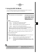
1-1 Using the DIFF EQ Mode 1. Using the DIFF EQ Mode You can solve differential equations numerically and graph the solutions. The general procedure for solving a differential equation is described below. Set Up 1. From the Main Menu, enter the DIFF EQ Mode. Execution 2. Select the differential equation type. • 1(1st) ........ Four types of first order differential equations • 2(2nd) ...... Second order linear differential equations • 3(N-th) ......
PAGE 3
1-2 Using the DIFF EQ Mode 6. Specify variables to graph or to store in LIST. Press 5(SET) and select c(Output) to display the list setting screen. x, y, y(1), y(2), ....., y(8) stand for the independent variable, the dependent variable, the first order derivative, the second order derivative, ....., and the eighth order derivative, respectively. 1st, 2nd, 3rd, ...., 9th stand for the initial values in order. To specify a variable to graph, select it using the cursor keys (f, c) and press 1(SEL).
PAGE 4
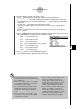
2-1 Differential Equations of the First Order 2. Differential Equations of the First Order k Separable Equation Description To solve a separable equation, simply input the equation and specify the initial values. dy/dx = f(x)g(y) Set Up 1. From the Main Menu, enter the DIFF EQ Mode. Execution 2. Press 1(1st) to display the menu of first order differential equations, and then select b(Separ). 3. Specify f(x) and g(y). 4. Specify the initial value for x0, y0. 5. Press 5(SET)b(Param). 6.
PAGE 5
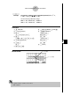
2-2 Differential Equations of the First Order ○ ○ ○ ○ ○ Example To graph the solutions of the separable equation dy/dx = y2 –1, x0 = 0, y0 = {0, 1}, –5 < x < 5, h = 0.1. Use the following V-Window settings. Xmin = –6.2, Xmax = 6.2, Xscale = 1 Ymin = –3.1, Ymax = 3.1, Yscale = 1 Procedure 1 m DIFF EQ 8 5(SET)c(Output)4(INIT)i 2 1(1st)b(Separ) 9 !K(V-Window) 3 bw a-(Y)Mc-bw 4 aw !*( { )a,b!/( } )w 5 5(SET)b(Param) 6 -fw fw -g.cw g.cw bwc -d.bw d.bw bwi 0 6(CALC) 7 a.
PAGE 6
2-3 Differential Equations of the First Order k Linear Equation To solve a linear equation, simply input the equation and specify initial values. dy/dx + f(x)y = g(x) Set Up 1. From the Main Menu, enter the DIFF EQ Mode. Execution 2. Press 1(1st) to display the menu of differential equations of the first order, and then select c(Linear). 3. Specify f(x) and g(x). 4. Specify the initial value for x0, y0. 5. Press 5(SET)b(Param). 6. Specify the calculation range. 7. Specify the step size for h. 8.
PAGE 7
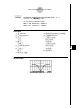
2-4 Differential Equations of the First Order ○ ○ ○ ○ ○ Example To graph the solution of the linear equation dy/dx + xy = x, x0 = 0, y0 = –2, –5 < x < 5, h = 0.1. Use the following V-Window settings. Xmin = –6.2, Xmax = 6.2, Xscale = 1 Ymin = –3.1, Ymax = 3.1, Yscale = 1 Procedure 1 m DIFF EQ 8 5(SET)c(Output)4(INIT)i 2 1(1st)c(Linear) 9 !K(V-Window) 3 vw vw 4 aw -cw 5 5(SET)b(Param) 6 -fw fw 7 a.bwi Result Screen -g.cw g.cw bwc -d.bw d.
PAGE 8
2-5 Differential Equations of the First Order k Bernoulli equation To solve a Bernoulli equation, simply input the equation and specify the power of y and the initial values. dy/dx + f(x)y = g(x)y n Set Up 1. From the Main Menu, enter the DIFF EQ Mode. Execution 2. Press 1(1st) to display the menu of differential equations of the first order, and then select d(Bern). 3. Specify f(x), g(x), and n. 4. Specify the initial value for x0, y0. 5. Press 5(SET)b(Param). 6. Specify the calculation range. 7.
PAGE 9
2-6 Differential Equations of the First Order ○ ○ ○ ○ ○ Example To graph the solution of the Bernoulli equation dy/dx – 2y = –y2, x0 = 0, y0 = 1, –5 < x < 5, h = 0.1. Use the following V-Window settings. Xmin = –6.2, Xmax = 6.2, Xscale = 1 Ymin = –3.1, Ymax = 3.1, Yscale = 1 Procedure 1 m DIFF EQ 7 a.bwi 2 1(1st)d(Bern) 8 5(SET)c(Output)4(INIT)i 3 -cw 9 !K(V-Window) -bw -g.cw cw g.cw 4 aw bw bwc -d.bw 5 5(SET)b(Param) d.
PAGE 10
2-7 Differential Equations of the First Order k Others To solve a general differential equation of the first order, simply input the equation and specify the initial values. Use the same procedures as those described above for typical differential equations of the first order. dy/dx = f(x, y) Set Up 1. From the Main Menu, enter the DIFF EQ Mode. Execution 2. Press 1(1st) to display the menu of differential equations of the first order, and then select e(Others). 3. Specify f(x, y). 4.
PAGE 11
2-8 Differential Equations of the First Order ○ ○ ○ ○ ○ Example To graph the solution of the first order differential equation dy/dx = – cos x, x0 = 0, y0 = 1, –5 < x < 5, h = 0.1. Use the following V-Window settings. Xmin = –6.2, Xmax = 6.2, Xscale = 1 Ymin = –3.1, Ymax = 3.1, Yscale = 1 Procedure 1 m DIFF EQ 8 5(SET)c(Output)4(INIT)i 2 1(1st)e(Others) 9 !K(V-Window) 3 -cvw -g.cw 4 aw g.cw bw bwc 5 5(SET)b(Param) -d.bw 6 -fw d.bw fw 7 a.
PAGE 12
3-1 Linear Differential Equations of the Second Order 3. Linear Differential Equations of the Second Order Description To solve a linear differential equation of the second order, simply input the equation and specify the initial values. Slope fields are not displayed for a linear differential equation of the second order. y앨 + f(x) y쎾 + g(x)y = h(x) Set Up 1. From the Main Menu, enter the DIFF EQ Mode. Execution 2. Press 2(2nd). 3. Specify f(x), g(x), and h(x). 4.
PAGE 13
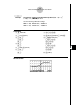
3-2 Linear Differential Equations of the Second Order ○ ○ ○ ○ ○ Example To graph the solution of the linear differential equation of the second order y앨 + 9y = sin 3x, x0 = 0, y0= 1, y쎾0 = 1, 0 < x < 10, h = 0.1. Use the following V-Window settings. Xmin = –1, Xmax = 11, Xscale = 1 Ymin = –3.1, Ymax = 3.1, Yscale = 1 Procedure 1 m DIFF EQ 8 5(SET)c(Output)4(INIT)i 2 2(2nd) 9 !K(V-Window) 3 aw -bw jw bbw sdvw bwc -d.bw 4 aw bw d.bw bw bw*2i 5 5(SET)b(Param) 0 6(CALC) 6 aw baw 7 a.
PAGE 14
4-1 Differential Equations of the Nth Order 4. Differential Equations of the Nth Order You can solve differential equations of the first through ninth order. The number of initial values required to solve the differential equation depends on its order. • Enter dependent variables y, y쎾, y앨, y(3), ....., y(9) as follows. a-(Y) 3(y(n))b(Y1) 3(y(n))c(Y2) 3(y(n))d(Y3) … y .................... y쎾 ................... y앨 ................... y(3)(=y쎾앨) ......... y(8) ................. 3(y(n))i(Y8) y(9) ........
PAGE 15
4-2 Differential Equations of the Nth Order ○ ○ ○ ○ ○ Example To graph the solution of the differential equation of the fourth order below y(4) = 0, x0 = 0, y0 = 0, y쎾0 = –2, y앨0 = 0, y(3)0 = 3, –5 < x < 5, h = 0.1. Use the following V-Window settings. Xmin = –6.2, Xmax = 6.2, Xscale = 1 Ymin = –3.1, Ymax = 3.1, Yscale = 1 Procedure 1 m DIFF EQ 9 5(SET)c(Output)4(INIT)i 2 3(N-th) 0 !K(V-Window) 3 3( n )ew -g.cw 4 aw g.cw 5 aw bwc aw -d.bw -cw d.
PAGE 16
4-3 Differential Equations of the Nth Order k Converting a High-order Differential Equation to a System of the First Order Differential Equations You can convert a single N-th order differential equation to a system of n first order differential equations. Set Up 1. From the Main Menu, enter the DIFF EQ Mode. Execution (N = 3) 2. Press 3(N-th). 3. Press 3(n)d to select a differential equation of the third order. 4. Perform substitutions as follows.
PAGE 17
4-4 Differential Equations of the Nth Order ○ ○ ○ ○ ○ Example Express the differential equation below as a set of first order differential equations. y(3) = sinx – y쎾 – y앨, x0 = 0, y0 = 0, y쎾0 = 1, y앨0 = 0. Procedure 1 m DIFF EQ 2 3(N-th) 3 3( n )dw 4 sv-3( y(n)) b-3( y(n))cw 5 aw aw bw aw 6 2(→SYS) 7 w(Yes) The differential equation is converted to a set of first order differential equations as shown below. (y1)쎾 = dy/dx = (y2) (y2)쎾 = d2y/dx2 = (y3) (y3)쎾 = sin x – (y2) – (y3).
PAGE 18
5-1 System of First Order Differential Equations 5. System of First Order Differential Equations A system of first order differential equations, for example, has dependent variables (y1), (y2), ....., and (y9), and independent variable x. The example below shows a system of first order differential equations. (y1)쎾= (y2) (y2)쎾= – (y1) + sin x Set Up 1. From the Main Menu, enter the DIFF EQ Mode. Execution 2. Press 4(SYS). 3. Enter the number of unknowns. 4. Enter the expression as shown below.
PAGE 19
5-2 System of First Order Differential Equations ○ ○ ○ ○ ○ Example 1 To graph the solution of first order differential equations with two unknowns below. (y1)쎾= (y2), (y2)쎾 = – (y1) + sin x, x0 = 0, (y1)0 = 1, (y2)0 = 0.1, –2 < x < 5, h = 0.1. Use the following V-Window settings.
PAGE 20
5-3 System of First Order Differential Equations ○ ○ ○ ○ ○ Example 2 To graph the solution of the system of first order differential equations below. (y1)쎾 = (2 – (y2)) (y1) (y2)쎾 = (2 (y1) – 3) (y2) x0 = 0, (y1)0 = 1, (y2)0 = 1/4, 0 < x < 10, h = 0.1. Use the following V-Window settings. Xmin = –1, Xmax = 11, Xscale = 1 Ymin = –1, Ymax = 8, Yscale = 1 Procedure 1 m DIFF EQ 9 5(SET)c(Output)4(INIT) 2 4(SYS) cc1( SEL) (Select ( y 1) and ( y 2) to graph.
PAGE 21
5-4 System of First Order Differential Equations k Further Analysis To further analyze the result, we can graph the relation between (y1) and (y2). Procedure 1 m STAT 2 List 1, List 2, and List 3 contain values for x, ( y 1), and ( y 2), respectively.
PAGE 22
5-5 System of First Order Differential Equations Important! • This calculator may abort calculation part way through when an overflow occurs part way through the calculation when calculated solutions cause the solution curve to extend into a discontinuous region, when a calculated value is clearly false, etc. • The following steps are recommended when the calculator aborts a calculation as described above. 1.