E ClassPad 330 ClassPad OS Version 3.05 User’s Guide CASIO Education website URL http://edu.casio.com ClassPad website URL http://edu.casio.com/products/classpad/ ClassPad register URL http://edu.casio.
GUIDELINES LAID DOWN BY FCC RULES FOR USE OF THE UNIT IN THE U.S.A. (not applicable to other areas). NOTICE This equipment has been tested and found to comply with the limits for a Class B digital device, pursuant to Part 15 of the FCC Rules. These limits are designed to provide reasonable protection against harmful interference in a residential installation.
1 Getting Ready Getting Ready This section contains important information you need to know before using the ClassPad for the first time. 1. Unpacking When unpacking your ClassPad, check to make sure that all of the items shown here are included. If anything is missing, contact your original retailer immediately. ClassPad CD-ROM Front Cover (Attached to ClassPad.) Stylus (Inserted in ClassPad.
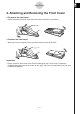
2 Getting Ready 2. Attaching and Removing the Front Cover S To remove the front cover Before using the ClassPad, remove the front cover and attach it to the back. S To attach the front cover When you are not using the ClassPad, attach the front cover to the front. Important! • Always attach the front cover to the ClassPad whenever you are not using it. Otherwise, accidental operation of the touch screen or the 0 key can cause the power to turn on and run down the batteries.
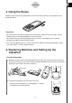
3 Getting Ready 3. Using the Stylus Slide the stylus from the slot provided for it on the ClassPad, and then use it to perform touch panel operations. Important! • Be careful so that you do not misplace or lose the stylus. When you are not using it, always keep the stylus in the slot provided for it on the ClassPad. • Be careful so that you do not damage the tip of the stylus. A damaged tip can scratch or otherwise damage the ClassPad touch panel.
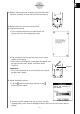
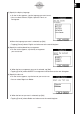
4 Getting Ready (3) Replace the battery cover, making sure that its tabs enter the holes marked and turn the ClassPad front side up. (4) Remove the front cover from the ClassPad. 2 (5) Align the touch panel. a. Your ClassPad should turn on automatically and display the Touch Panel Alignment screen. b. Tap the center of each of the four cross marks as they appear on the display. • If the Touch Panel Alignment screen does not appear, use the stylus to press the P button on the back of the ClassPad.
5 Getting Ready (7) Specify the display language. a. On the list that appears, tap the language you want to use. • You can select German, English, Spanish, French, or Portuguese. b. When the language you want is selected, tap [Set]. • Tapping [Cancel] selects English and advances to the next dialog box. (8) Specify the soft keyboard key arrangement. a. On the list that appears, tap the key arrangement you want to use. b. When the key arrangement you want is selected, tap [Set].
6 Getting Ready (10) Configure power properties. a. Configure the Power Save Mode and Auto Power Off settings. • See “Power Saving Mode” and “Auto Power Off” on page 16-6-1 for details about these settings. b. When the configurations are the way you want, tap [Set]. • Tapping [Cancel] selects “1 day” for [Power Save Mode] and “6 min” for [Auto Power Off], and finalizes the setup operation. 5.
7 Getting Ready Handling Precautions • Your ClassPad is made of precision components. Never try to take it apart. • Avoid dropping your ClassPad and subjecting it to strong impact. • Do not store the ClassPad or leave it in areas exposed to high temperatures or humidity, or large amounts of dust. When exposed to low temperatures, the ClassPad may require more time to display results and may even fail to operate. Correct operation will resume once the ClassPad is brought back to normal temperature.
8 Getting Ready Be sure to keep physical records of all important data! Low battery power or incorrect replacement of the batteries that power the ClassPad can cause the data stored in memory to be corrupted or even lost entirely. Stored data can also be affected by strong electrostatic charge or strong impact. It is up to you to keep back up copies of data to protect against its loss.
• • • • • • • • • • • • • • • • • • • • • • • • • • • • • • • • • • • • • • • • • • • • • • • • • • • • • • • • • • • • • • • • • • • • • • • • • • • • • • • • • • • • • • • • • • • • • • • • • • • • • • • • • • • • • • • • • • ClassPad 330 • • • • • • • • • • • • • • • • • • • • • • • • • • • • • • • • • • • • • • • • • • • • • • • • • • • • • • • • • • • • • • • • • • • • • • • • • • • • • • • • • • • • • • • • • • • • • • • • • • • • • • • • • • • • • • • • • • • • • • • • • • • •
1 Contents Contents Getting Ready 1. Unpacking .....................................................................................................1 2. Attaching and Removing the Front Cover .................................................2 3. Using the Stylus ...........................................................................................3 4. Replacing Batteries and Setting Up the ClassPad ....................................3 5. User Registration .............................................
2 Contents 1-7 Variables and Folders .......................................................................... 1-7-1 Folder Types.......................................................................................................1-7-1 Variable Types ...................................................................................................1-7-2 Creating a Folder ...............................................................................................1-7-4 Creating and Using Variables ....
3 Contents 2-6 Matrix and Vector Calculations ............................................................ 2-6-1 Inputting Matrix Data ..........................................................................................2-6-1 Performing Matrix Calculations...........................................................................2-6-4 Using a Matrix to Assign Different Values to Multiple Variables .........................2-6-6 2-7 Specifying a Number Base ............................................
4 Contents 2-12 Using Probability ................................................................................ 2-12-1 Starting Up Probability ......................................................................................2-12-2 Probability Menus and Buttons .........................................................................2-12-2 Using Probability...............................................................................................
5 Contents 3-7 Using Trace ............................................................................................ 3-7-1 Using Trace to Read Graph Coordinates ...........................................................3-7-1 Linking Trace to a Number Table .......................................................................3-7-3 Generating Number Table Values from a Graph ................................................3-7-4 3-8 Analyzing a Function Used to Draw a Graph ............................
6 Contents 5-5 Other 3D Graph Application Functions............................................... 5-5-1 Using Trace to Read Graph Coordinates ...........................................................5-5-1 Inserting Text into a 3D Graph Window..............................................................5-5-1 Calculating a z-value for Particular x- and y-values, or s- and t-values ..............5-5-2 Using Drag and Drop to Down a 3D Graph ........................................................
7 Contents 7-5 Graphing Paired-Variable Statistical Data........................................... 7-5-1 Drawing a Scatter Plot and xy Line Graph .........................................................7-5-1 Drawing a Regression Graph (Curve Fitting) .....................................................7-5-2 Graphing Previously Calculated Regression Results .........................................7-5-4 Drawing a Linear Regression Graph ..................................................................
8 Contents 8-3 Editing Figures ...................................................................................... 8-3-1 Selecting and Deselecting Figures .....................................................................8-3-1 Moving and Copying Figures ..............................................................................8-3-3 Pinning an Annotation on the Geometry Window ...............................................8-3-4 Specifying the Number Format of a Measurement .......................
9 Contents 10-4 Working with eActivity Files............................................................... 10-4-1 Opening an Existing eActivity ...........................................................................10-4-1 Browsing the Contents of an eActivity ..............................................................10-4-2 Editing the Contents of an eActivity ..................................................................10-4-2 Expanding an Application Data Strip ...............................
10 Contents 12-3 Debugging a Program ......................................................................... 12-3-1 Debugging After an Error Message Appears....................................................12-3-1 Debugging a Program Following Unexpected Results .....................................12-3-1 Modifying an Existing Program to Create a New One ......................................12-3-2 Searching for Data Inside a Program ...............................................................
11 Contents Paste ..............................................................................................................13-4-11 Specifying Text or Calculation as the Data Type for a Particular Cell ............13-4-13 Using Drag and Drop to Copy Cell Data within a Spreadsheet ......................13-4-14 Using Drag and Drop to Obtain Spreadsheet Graph Data .............................13-4-16 Recalculating Spreadsheet Expressions ........................................................
12 Contents 14-5 Drawing f(x) Type Function Graphs and Parametric Function Graphs.................................................................................................. 14-5-1 Drawing an f (x) Type Function Graph ..............................................................14-5-1 Drawing a Parametric Function Graph .............................................................14-5-2 14-6 Configuring Differential Equation Graph View Window Parameters .............................................
13 Contents 15-8 Day Count ............................................................................................ 15-8-1 Day Count Fields ..............................................................................................15-8-1 Financial Application Default Setup for Examples ............................................15-8-1 15-9 Depreciation ........................................................................................ 15-9-1 Depreciation Fields ...............................
14 Contents 16-6 Configuring Power Properties ........................................................... 16-6-1 Power Saving Mode .........................................................................................16-6-1 Auto Power Off .................................................................................................16-6-1 Configuring Power Properties...........................................................................
0 0-1-1 About This User’s Guide About This User’s Guide This section explains the symbols that are used in this user’s guide to represent keys, stylus operations, display elements, and other items you encounter while operating your ClassPad. ClassPad Keypad and Icon Panel Icon panel s m M r S h Cursor key Keyboard ON/OFF Clear = Keypad x ( ) , (–) y z 7 4 1 0 8 5 2 .
0-1-2 About This User’s Guide On-screen Keys, Menus, and Other Controllers Menu bar Toolbar Tabs Soft keyboard Menu bar Menu names and commands are indicated in text by enclosing them inside of brackets. The following examples show typical menu operations. Example 1: Tap the menu and then tap [Keyboard]. Example 2: Tap [Analysis], [Sketch], and then [Line].
0-1-3 About This User’s Guide Toolbar Toolbar button operations are indicated by illustrations that look like the button you need to tap. Example 1: Tap to graph the functions. Example 2: Tap to open the Stat Editor window. Soft keyboard Key operations on the soft keyboards that appear when you press the . key are indicated by illustrations that look like the keyboard keys. You can change from one keyboard type to another by tapping one of the tabs along the top of the soft keyboard.
Chapter Getting Acquainted 1-1 1-2 1-3 1-4 1-5 1-6 1-7 1-8 1-9 General Guide Turning Power On and Off Using the Icon Panel Built-in Applications Built-in Application Basic Operations Input Variables and Folders Using the Variable Manager Configuring Application Format Settings 20060301 1
1-1-1 General Guide 1-1 General Guide Front Side s m M rS h Keyboard Clear = ( ON/OFF ) , (–) x 7 4 1 0 y z 8 5 2 .
1-1-2 General Guide General Guide The numbers next to each of the items below correspond to the numbers in the illustration on page 1-1-1. Front Touch screen The touch screen shows calculation formulas, calculation results, graphs and other information. The stylus that comes with the ClassPad can be used to input data and perform other operations by tapping directly on the touch screen. Stylus This stylus is specially designed for performing touch screen operations.
1-1-3 General Guide Keypad Use these keys to input the values and operators marked on them. See “1-6 Input” for details. key Press this key to execute a calculation operation or enter a return. Side 3-pin data communication port Connect the data communication cable here to communicate with another ClassPad unit or a CASIO Data Analyzer. See “Chapter 17 – Performing Data Communication” for details. 4-pin mini USB port Connect the data communication cable here to exchange data with a computer.
1-1-4 General Guide Using the Stylus Most value and formula input, command executions, and other operations can be performed using the stylus. I Things you can do with the stylus Tap Drag • This is equivalent to clicking with a mouse. • To perform a tap operation, tap lightly with the stylus on the ClassPad’s touch screen. • Tapping is used to display a menu, execute an on-screen button operation, make a window active, etc. • This is equivalent to dragging with a mouse.
1-2-1 Turning Power On and Off 1-2 Turning Power On and Off Turning Power On You can turn on the ClassPad either by pressing the 0 key or by tapping the touch screen with the stylus. • Turning on the ClassPad (while it is in the sleep state) displays the window that was on the display when you last turned it off. See “Resume Function” below. • Note that you need to perform a few initial setup operations when you turn on the ClassPad the first time after purchasing it.
1-2-2 Turning Power On and Off Limiting the Duration of the Sleep State You can use the [Power Save Mode] setting (page 16-6-1) to limit the duration of the sleep state that is entered by the Resume function. If you have “1 day” specified for [Power Save Mode], for example, the ClassPad remains in the sleep state for one day after power is turned off. After that, the ClassPad powers down completely, which deletes all data that was backed up by the Resume function.
1-3-1 Using the Icon Panel 1-3 Using the Icon Panel The icon panel of seven permanent icons is located below the touch screen. Tapping an icon executes the function assigned to it. The table below explains what you can do with the icon panel icons. Function When you want to do this: Tap this icon: Display the menu to configure settings, switch to the application menu, etc. See “Using the Menu” on page 1-5-4. 3 Display the application menu See “1-4 Built-in Applications” for details.
1-4-1 Built-in Applications 1-4 Built-in Applications Tapping / on the icon panel displays the application menu. The table below shows the icon menu names of the built-in applications, and explains what you can do with each application.
1-4-2 Built-in Applications To perform this type of operation: • Exchange data with another ClassPad, a computer, or another device • Clear the memory • Adjust contrast • Configure other system settings Select this icon: See Chapter: 17 & 16 Starting a Built-in Application Perform the steps below to start a built-in application. S ClassPad Operation (1) On the icon panel, tap / to display the application menu.
1-4-3 Built-in Applications • Displaying applications according to group (Additional Applications, All Applications) See “Using Application Groups” below. • Moving or swapping icons See “Moving an Icon” below, and “Swapping Two Icons” on page 1-4-4. • Deleting an application See “Deleting an Application” on page A-2-1. I Using Application Groups You can use application groups to specify the type of applications that appear on the application menu.
1-4-4 Built-in Applications S ClassPad Operation (1) On the icon panel, tap / to display the application menu. (2) Tap at the top left of the application menu. • This opens a menu of setting options. (3) Tap [Move Icon]. (4) Tap the icon you want to move ( in this example). • This selects the icon. (5) Tap the icon that you want the first icon to follow ( in this example). • This moves the icon. I Swapping Two Icons Perform the following steps to swap two icons on the application menu.
1-5-1 Built-in Application Basic Operations 1-5 Built-in Application Basic Operations This section explains basic information and operations that are common to all of the built-in applications. Application Window The following shows the basic configuration of a built-in application window.
1-5-2 Built-in Application Basic Operations When using two windows, the currently selected window (the one where you can perform operations) is called the “active window”. The menu bar, toolbar, and status bar contents are all applicable to the active window. The active window is indicated by a thick boundary around it. S To switch the active window While a dual window is on the display, tap anywhere inside the window that does not have a thick boundary around it to make it the active window.
1-5-3 Built-in Application Basic Operations Using the Menu Bar The menu bar appears along the top of the window of each application. It shows the menus that you can access for the currently active window. } Menu bar Tapping the menu bar menu displays its commands, options, and settings from which you can choose the one you want. Some menu items have a single selection as shown in Example 1, below, while other menu items display a submenu of selections from which you can choose as shown in Example 2.
1-5-4 Built-in Application Basic Operations Using the Menu The menu appears at the top left of the window of each application, except for the System application. You can access the menu by tapping 3 on the icon panel, or by tapping the menu bar’s menu. I Menu Items The following describes all of the items that appear on the menu. Tapping [Variable Manager] starts up the Variable Manager. See “1-8 Using the Variable Manager” for details.
1-5-5 Built-in Application Basic Operations I Using the Menu to Access Windows Most ClassPad applications support simultaneous display of two windows. When two windows are on the display, the one with a thick selection boundary around it is the active window. The displayed menu and toolbar are the ones for the currently active window. You can use the menu to change the active window and to display the window you want. S Window Selection Example (Graph & Table) E E (1) Graph window is active.
1-5-6 Built-in Application Basic Operations Using Check Boxes A check box shows the current status of a dialog box option that can be turned on or off. An option is turned on (selected) when its check box has a check mark inside it. An option is turned off when a check box is cleared. Tapping a check box toggles the option on (checked) and off (cleared). Option turned on Option turned off Check boxes also appear on menus. Menu check boxes operate the same way as dialog box check boxes.
1-5-7 Built-in Application Basic Operations Using Option Buttons Option buttons are used on dialog boxes that present you with a list of options from which you can select only one. A black option button indicates the currently selected option, while the buttons of the options that are not selected are white. Tap “Français”. This selects “Français” and deselects “English”. Option buttons also appear on menus. Menu option buttons operate the same way as dialog box option buttons.
1-5-8 Built-in Application Basic Operations Using the Toolbar The toolbar is located directly underneath the menu bar of an application window. It contains the buttons for the currently active window. } Toolbar I Toolbar Buttons Normally, you tap a button to execute the command assigned to it. Some buttons, however, have a down arrow 6 next to them. Tapping the arrow displays a list of options from which you can select.
1-5-9 Built-in Application Basic Operations Interpreting Status Bar Information The status bar appears along the bottom of the window of each application. Status bar Information about current application Tip • You can change the configuration of a setting indicated in the status bar by tapping it. Tapping “Cplx” (indicating complex number calculations) while the Main application is running will toggle the setting to “Real” (indicating real number calculations).
1-5-10 Built-in Application Basic Operations Example: To pause a graphing operation and then resume it ClassPad Operation S\ (1) Use the Graph & Table application to draw a graph. • For details about graphing, see “Chapter 3 – Using the Graph & Table Application”. (2) While the graph is being drawn, press the key. • This pauses the draw operation and displays the right side of the status bar. on Draw is paused at the point where is pressed. (3) To resume the operation, press the key again.
1-6-1 Input 1-6 Input You can input data on the ClassPad using its keypad or by using the on-screen soft keyboard. Virtually all data input required by your ClassPad can be performed using the soft keyboard. The keypad keys are used for input of frequently used data like numbers, arithmetic operators, etc. Using the Soft Keyboard The soft keyboard is displayed in the lower part of the touch screen. A variety of different special-purpose soft keyboard styles help to take much of the work out of data input.
1-6-2 Input I Soft Keyboard Styles There are four different soft keyboard styles as described below. • Math (mth) Keyboard Pressing . will display the keyboard that you last displayed while working in that application. If you quit the application and go into another application, then the (default) soft keyboard appears. You can use the math (mth) keyboard to input values, variables, and expressions. Tap each lower button to see additional characters, for example tap .
1-6-3 Input I Selecting a Soft Keyboard Style Tap one of the tabs along the top of the soft keyboard ( , , the keyboard style you want. , or ) to select Tap here. To display the 2D keyboard Input Basics This section includes a number of examples that illustrate how to perform basic input procedures. All of the procedures assume the following. • The Main application is running. For details, see “Starting a Built-in Application” on page 1-4-2. • The soft keyboard is displayed.
1-6-4 Input Example 2: To simplify 2 (5 + 4) w (23 s 5) S ClassPad Operation Using the keypad keys ;;* Using the soft keyboard Tap the keys of the math (mth) keyboard or the 2D keyboard to input the calculation expression. ;* (or ) A D C AB D U Tip • As shown in Example 1 and Example 2, you can input simple arithmetic calculations using either the keypad keys or the soft keyboard.
1-6-5 Input S To delete an unneeded key operation Use B and C to move the cursor to the location immediately to the right of the key operation you want to delete, and then press . Each press of deletes one command to the left of the cursor. Example: To change the expression 369 s s 2 to 369 s 2 (1) * (2) B Tip • You can move the cursor without using the cursor key by tapping at the destination with the stylus. This causes the cursor to jump to the location where you tap.
1-6-6 Input S To insert new input into the middle of an existing calculation expression Use B or C to move the cursor to the location where you want to insert new input, and then input what you want. Example: To change 2.362 to sin(2.362) (1) * A BEV (2) BBBBBB (3) 3Q Tip • You can move the cursor without using the cursor key by tapping at the destination with the stylus. This causes the cursor to jump to the location where you tap.
1-6-7 Input I Using the Clipboard for Copy and Paste You can copy (or cut) a function, command, or other input to the ClassPad’s clipboard, and then paste the clipboard contents at another location. S To copy characters (1) Drag the stylus across the characters you want to copy to select them. (2) On the soft keyboard, tap &. • This puts a copy of the selected characters onto the clipboard. The selected characters are not changed when you copy them.
1-6-8 Input Copying and pasting in the message box S\ The “message box” is a 1-line input and display area under the Graph window (see Chapter 3). Message box You can use the two buttons to the right of the message box to copy the message box contents (& button), or to paste the clipboard contents to the message box (' button). Copy and paste are performed the same way as the copy and paste operations using the soft keyboard.
1-6-9 Input S 3 key set Tapping the 3 key displays keys for inputting trigonometric functions, and changes the 3 softkey to (. You can tap this key to toggle between 3 and the default keyboard. Tapping the (hyperbolic) key switches to a key set for inputting hyperbolic functions. Tap the key again to return to the regular 3 key set. k m S key set Tapping the key displays keys for inputting differential and integral calculus expressions, permutations, etc., and changes the softkey to (.
1-6-10 Input S 5 key set Tapping the 5 key displays keys for inputting single-character variables, and changes the 5 softkey to (. You can tap this key to toggle between 5 and the default keyboard. Tapping the $ key switches to a key set for inputting upper-case singlecharacter variables. k$m Tip • As its name suggests, a single-character variable is a variable name that consists of a single character like “a” or “x”. Each character you input on the 5 keyboard is treated as a singlecharacter variable.
1-6-11 Input S , key set Use the , key set to input Greek characters, Cyrillic characters, and accented characters. Tap the ) and * buttons to scroll to additional keys. Tapping $ caps locks the keyboard for input of upper-case characters. • Tap ( to return to the initial alphabet (abc) key set. S L key set This key set contains some of the mathematical expression symbols that are also available on the math (mth) keyboard. Tap the ) and * buttons to scroll to additional keys.
1-6-12 Input I Using Single-character Variables As its name suggests, a single-character variable is a variable name that consists of a single character like “a” or “x”. Input of single-character variable names is subject to different rules than input of a series of multiple characters (like “abc”). S To input a single-character variable name Any character you input using any one of the following techniques is always treated as a single-character variable.
1-6-13 Input S To input a series of multiple characters A series of multiple characters (like “list1”) can be used for variable names, program commands, comment text, etc. Always use the alphabet (abc) keyboard when you want to input a series of characters. Example: ?@AU You can also use the alphabet (abc) keyboard to input single-character variable names. To do so, simply input a single character, or follow a single character with a mathematical operator.
1-6-14 Input S Catalog (cat) keyboard configuration This is an alphabetized list of commands, functions, and other items available in the category currently selected with “Form”. Tap the down button and then select the category you want ([Func], [Cmd], [Sys], [User], or [All]) from the list that appears. Tapping a letter button displays the commands, functions, or other items that begin with that letter. Tap this key to input the item that is currently selected in the alphabetized list.
1-6-15 Input I Using the 2D Keyboard The 2D keyboard provides you with a number of templates that let you input fractions, exponential values, nth roots, matrices, differentials, integrals, and other complex expressions as they appear in your textbook. It also includes a 5 key set that you can use to input single-character variables like the ones you can input with the math (mth) keyboard. S Initial 2D keyboard key set This key set lets you input fractions, exponential values, nth roots, etc.
1-6-16 Input To input this: Use these keys: For more information, see: “0” under “Using the Calculation Submenu” on page 2-8-15. Sum of product template Differential coefficient template Integration template S ADV , / “diff” under “Using the Calculation Submenu” on page 2-8-13. “°” under “Using the Calculation Submenu” on page 2-8-14. key set Tapping the place of the ADV ADV key displays a keyboard like the one shown below, which has a ( key in key. Tapping ( returns to the initial 2D keyboard.
1-6-17 Input S 5 key set Tapping the 5 key displays keys for inputting single-character variables, and changes the 5 softkey to (. You can tap this key to toggle between 5 and the initial 2D keyboard. Tapping the $ key switches to a key set for inputting upper-case single-character variables. k$m Tip • As its name suggests, a single-character variable is a variable name that consists of a single character like “a” or “x”.
1-6-18 Input Tip • If you want your ClassPad to evaluate a calculation expression and display a result in the eActivity application, you must input the calculation in a calculation row. See “Inserting a Calculation Row” on page 10-3-3. n Example 2: To input k=1 k2 (1) Tap to display the 2D keyboard and then tap (2) Tap . . Initially, the cursor appears here. (3) In the input box below 3, input “k=1”.
1-6-19 Input (4) Tap with the stylus to move the cursor to the other input locations to enter the limits of integration. In the input box above °, tap @. In the input box below °, tap ?. (5) After everything is the way you want, press .
1-7-1 Variables and Folders 1-7 Variables and Folders Your ClassPad lets you register text strings as variables. You can then use a variable to store a value, expression, string, list, matrix, etc. A variable can be recalled by a calculation to access its contents. Variables are stored in folders. In addition to the default folders that are provided automatically, you can also create your own user folders. You can create user folders as required to group variables by type or any other criteria.
1-7-2 Variables and Folders I Current Folder The current folder is the folder where the variables created by applications (excluding eActivity) are stored and from which such variables can be accessed. The initial default current folder is the “main” folder. You can also select a user folder you created as the current folder. For more information about how to do this, see “Specifying the Current Folder” on page 1-8-3.
1-7-3 Variables and Folders I Variable Data Types ClassPad variables support a number of data types. The type of data assigned to a variable is indicated by a data type name. Data type names are shown on the Variable Manager variable list, and on the Select Data dialog box that appears when you are specifying a variable in any ClassPad application. The following table lists all of the variable data type names and explains the meaning of each.
1-7-4 Variables and Folders Creating a Folder You can have up to 87 user folders in memory at the same time. This section explains how to create a user folder and explains the rules that cover folder names. You can create a folder using either the Variable Manager or the “NewFolder” command. I Creating a folder using the Variable Manager On the Variable Manager window, tap [Edit] and then [Create Folder]. For more information, see “1-8 Using the Variable Manager”.
1-7-5 Variables and Folders (4) Tap U to execute the command. • The message “done” appears on the display to let you know that command execution is complete. Tip • You can use the Variable Manager to view the contents of a folder you create. For more information, see “1-8 Using the Variable Manager”. • For information about commands you can use to perform folder operations, see “12-6 Program Command Reference”. I Folder Name Rules The following are the rules that apply to folder names.
1-7-6 Variables and Folders I Single-character Variable Precautions Your ClassPad supports the use of single-character variables, which are variables whose names consist of a single character like “a” or “x”. Some ClassPad keys (7, 8, ' keypad keys, math (mth) soft keyboard 7, 8, 9, : keys, 5 key set keys, etc.) are dedicated single-character variable name input keys. You cannot use such a key to input a variable name that has more than one character.
1-7-7 Variables and Folders Tip • As shown in the above example, assigning something to a variable with a name that does not yet exist in the current folder causes a new variable with that name to be created. If a variable with the specified name already exists in the current folder, the contents of the existing variable are replaced with the newly assigned data, unless the existing variable is protected. For more information about protected variables, see “Protected variable types” on page 1-7-3.
1-7-8 Variables and Folders I “library” Folder Variables Variables in the “library” folder can be accessed without specifying a path name, regardless of the current folder. Example: To create and access two variables, one located in the “library” folder and one located in another folder S ClassPad Operation (1) With “main” specified as the current folder (the default), perform the following operation to create a variable named “eq1” and assign the indicated list data to it.
1-7-9 Variables and Folders eq2 U Since variable “eq2” is stored in the “library” folder, you do not need to indicate a path to access it. Tip • Specifying a variable name that exists in both the current folder and the “library” folder causes the variable in the current folder to be accessed. For details about the variable access priority sequence and how to access variables in particular folders, see “Rules Governing Variable Access” on page 1-7-11.
1-7-10 Variables and Folders Assigning Values and Other Data to a System Variable As its name suggests, a system variable is a variable that is created and used by the system (page 1-7-5). Some system variables allow you to assign values and other data to them, while some system variables do not. For more information about which variables allow you to control their contents, see the “System Variable Table” on page A-7-1.
1-7-11 Variables and Folders Rules Governing Variable Access Normally, you access a variable by specifying its variable name. The rules in this section apply when you need to reference a variable that is not located in the current folder or to access a variable that has the same name as one or more variables located in other folders. I Variable Search Priority Sequence Specifying a variable name to access a variable, searches variables in the following sequence.
1-8-1 Using the Variable Manager 1-8 Using the Variable Manager The Variable Manager is a tool for managing user variables, programs, user functions, and other types of data. Though this section uses only the term “variables”, the explanations provided here also refer to the other types of data that can be managed by the Variable Manager. Variable Manager Overview This section explains how to start up and exit the Variable Manager.
1-8-2 Using the Variable Manager Variable Manager Views The Variable Manager uses two views, a folder list and a variable list. • The folder list always appears first whenever you start up the Variable Manager. Current folder Number of variables contained in the folder Folder names Folder List • Tapping a folder name on the folder list selects it. Tapping the folder name again displays the folder’s contents; a variable list.
1-8-3 Using the Variable Manager Variable Manager Folder Operations This section describes the various folder operations you can perform using the Variable Manager. I Specifying the Current Folder The “current folder” is the folder where the variables created by applications (excluding eActivity) are stored and from which such variables can be accessed. The initial default current folder is the “main” folder. You can also select a folder you created yourself as the current folder.
1-8-4 Using the Variable Manager I Selecting and Deselecting Folders The folder operations you perform are performed on the currently selected folders. The folders that are currently selected on the folder list are those whose check boxes are selected (checked). You can use the following operations to select and deselect folders as required. To do this: Do this: Select a single folder Select the check box next to the folder name. Deselect a single folder Clear the check box next to the folder name.
1-8-5 Using the Variable Manager Tip • You cannot delete the “library” folder or the “main” folder. • If no check box is currently selected on the folder list, the folder whose name is currently highlighted on the list is deleted when you tap [Edit] and then [Delete]. • An error message appears and the folder is not deleted if any one of the following conditions exists. • The folder is locked. • Any variable inside the folder is locked. • There are still variables inside the folder.
1-8-6 Using the Variable Manager I Inputting a Folder Name into an Application Perform the procedure below when you want to input the name of a folder displayed on the Variable Manager window into the application from which you started up the Variable Manager. ClassPad Operation S\ (1) In the Main application, Graph & Table application, or some other application, move the cursor to the location where you want to input the folder name. (2) Start up the Variable Manager to display the list of folders.
1-8-7 Using the Variable Manager Variable Operations This section explains the various operations you can perform on the Variable Manager variables. I Opening a Folder Perform the steps below to open a folder and display the variables contained inside it. S ClassPad Operation (1) Start up the Variable Manager and display the folder list. (2) Tap the name of the folder you want to open so it is highlighted, and then tap it again. • This opens the folder and displays a variable list showing its contents.
1-8-8 Using the Variable Manager (3) On the dialog box, tap the down arrow button and then select the data type from the list that appears. • To display variables for all data types, select [All]. • For details about data type names and variables, see “Variable Data Types” on page 1-7-3. (4) After selecting the data type you want, tap [OK] to apply it or [Cancel] to exit the selection dialog box without changing the current setting.
1-8-9 Using the Variable Manager I Deleting a Variable Perform the following steps when you want to delete a variable. S ClassPad Operation (1) Open the folder that contains the variable you want to delete and display the variable list. (2) Select the check box next to the variable you want to delete. • To delete multiple variables, select all of their check boxes. (3) Tap [Edit] and then [Delete].
1-8-10 Using the Variable Manager Tip • If no check box is currently selected on the variable list, the variable whose name is currently highlighted on the list is copied or moved. • If a variable with the same name already exists in the destination folder, the variable in the destination folder is replaced with the one that you are copying or moving.
1-8-11 Using the Variable Manager S To unlock a variable (1) Open the folder that contains the variable you want to unlock and display the variable list. (2) Select the check box next to the variable you want to unlock. (3) Tap [Edit] and then [Unlock]. I Searching for a Variable You can use the following procedure to search the “main” folder or a user defined folder for a particular variable name. Note that you cannot search the “library” folder.
1-8-12 Using the Variable Manager I Viewing the Contents of a Variable You can use the Variable Manager to view the contents of a particular variable. ClassPad Operation S\ (1) Open the folder that contains the variable whose contents you want to view and display on the variable list. (2) Tap the name of the variable whose contents you want to view so it is highlighted, and then tap it again. • This displays a dialog box that shows the contents of the variable.
1-8-13 Using the Variable Manager I Inputting a Variable Name into an Application Perform the procedure below when you want to input the name of a variable from the Variable Manager window into the application from which you started up the Variable Manager. ClassPad Operation S\ (1) In the Main application, Graph & Table application, or some other application, move the cursor to the location where you want to input the variable name. (2) Start up the Variable Manager to display the folder list.
1-9-1 Configuring Application Format Settings 1-9 Configuring Application Format Settings The menu includes format settings for configuring the number of calculation result display digits and the angle unit, as well as application-specific commands. The following describes each of the settings and commands that are available on the menu.
1-9-2 Configuring Application Format Settings Specifying a Variable Certain settings require that you specify variables. If you specify a user-stored variable when configuring the setting of such an item, you must specify the folder where the variable is stored and the variable name. Example: To use [Table Variable] on the [Special] tab of the Graph Format dialog box for configuring a user variable ClassPad Operation S\ (1) Tap , or tap 3 on the icon panel, and then tap [Graph Format].
1-9-3 Configuring Application Format Settings (5) Use the Select Data dialog box to specify the folder where the variable is saved, and then specify the variable name. • The sample dialog box in step (4) shows selection of the list variable named “ab”, which is located in the folder named “main”. (6) Tap [OK]. • This closes the Select Data dialog box. This line shows the \ specified in step (5) (“main\ab” in this case).
1-9-4 Configuring Application Format Settings Application Format Settings This section provides details about all of the settings you can configure using the application format settings. The following two points apply to all of the dialog boxes. • Some settings involve turning options on or off. Selecting a check box next to an option (so it has a check mark) turns it on, while clearing the check box turns it off. • Other settings consist of a text box with a down arrow button on the right.
1-9-5 Configuring Application Format Settings S Number Format To specify this type of numeric value display format: Auto exponential display for values less than 10–2 and from 1010 or greater (when you are in the Decimal mode) Auto exponential display for values less than 10–9 and from 1010 or greater (when you are in the Decimal mode) Fixed number of decimal places Fixed number of significant digits Select this setting: Normal 1* Normal 2 Fix 0 – 9 Sci 0 – 9 S Angle To specify this angle unit: Radians D
1-9-6 Configuring Application Format Settings *1 Executing 1 w 2 in the Decimal mode produces a result of 0.5, while the Standard mode produces a result of 1 . 2 *2 Executing x2 + 2x + 3x + 6 in the Assistant mode produces a result of x2 + 2 • x + 3 • x + 6, while the Algebra mode produces a result of x2 + 5 • x + 6. Important! The Assistant mode is available in the Main application and eActivity application only.
1-9-7 Configuring Application Format Settings To do this: Do this: Turn off display of graph controller arrows during graphing Clear the [G-Controller] check box.* Draw graphs with plotted points Select the [Draw Plot] check box. Draw graphs with solid lines Clear the [Draw Plot] check box.* Turn on display of function name and function Select the [Graph Function] check box.* Turn off display of function name and function Clear the [Graph Function] check box.
1-9-8 Configuring Application Format Settings S Summary Table To specify this source for summary table data: Select this setting: View Window View Window* List data list1 through list6 Select list data to be used as source for summary table data S Summary Table f ’’(x) To do this: Select this setting: Turn on display of second derivative for summary tables On* Turn off display of second derivative for summary tables Off S Stat Window Auto To do this: Do this: Configure Statistic
1-9-9 Configuring Application Format Settings S Labels To do this: Select this setting: Turn on display of Graph window axis labels On Turn off display of Graph window axis labels Off* S Background To do this: Select this setting: Turn off Graph window background display Off* Select an image to be used as the Graph window background • The above is the same as the [Background] setting on the Graph Format dialog box.
1-9-10 Configuring Application Format Settings S Number Format To specify this type of numeric value display format on the Geometry window: Select this setting: Auto exponential display for values less than 10–2 and from 1010 or greater (when you are in the Decimal mode) Normal 1 Auto exponential display for values less than 10–9 and from 1010 or greater (when you are in the Decimal mode) Normal 2 Fixed number of decimal places Fix 0 – 9 Fixed number of significant digits Sci 0 – 9 • The initial
1-9-11 Configuring Application Format Settings I Advanced Format Dialog Box Use the Advanced Format dialog box to configure settings for Fourier transform and FFT settings.
1-9-12 Configuring Application Format Settings I Financial Format Dialog Box Use the Financial Format dialog box to configure settings for the Financial application.
1-9-13 Configuring Application Format Settings Special Tab S Odd Period To do this: Select this setting: Specify compound interest for odd (partial) months Compound (CI) Specify simple interest for odd (partial) months Simple (SI) Specify no separation of full and odd (partial) months Off* S Compounding Frequency To do this: Select this setting: Specify once a year compounding Annual* Specify twice a year compounding Semi-annual S Bond Interval To do this: Select this setting: Use a number
1-9-14 Configuring Application Format Settings I Presentation Dialog Box Use the Presentation dialog box to configure settings for the Presentation application. For full details about the Presentation application, see Chapter 11. To do this: Do this: Send hard copy data to an external device Select “Outer Device” for [Screen Copy To].* Save hard copy data internally as Presentation data Select “P1:**” through “P20:**” for [Screen Copy To].
1-9-15 Configuring Application Format Settings I Communication Dialog Box Use the Communication dialog box to configure communication settings. For full details about the Communication application, see Chapter 17.
Chapter Using the Main Application The Main application is a general-purpose numerical and mathematical calculation application that you can use to study mathematics and solve mathematical problems. You can use the Main application to perform general operations from basic arithmetic calculations, to calculations that involve lists, matrices, etc.
2-1-1 Main Application Overview 2-1 Main Application Overview This section provides information about the following. • Main application windows • Modes that determine how calculations and their results are displayed • Menus and their commands Starting Up the Main Application Use the following procedure to start up the Main application. S ClassPad Operation On the application menu, tap . This starts the Main application and displays the work area.
2-1-2 Main Application Overview • Basic Main application operations consist of inputting a calculation expression into the work area and pressing . This performs the calculation and then displays its result on the right side of the work area. Input expression Calculation result • Calculation results are displayed in natural format, with mathematical expressions appearing just as they do in your textbook. You can also input expressions in natural format using the soft keyboard.
2-1-3 Main Application Overview Main Application Menus and Buttons This section explains the operations you can perform using the menus and buttons of the Main application. • For information about the menu, see “Using the Menu” on page 1-5-4.
2-1-4 Main Application Overview Using Main Application Modes The Main application has a number of different modes that control how calculation results are displayed, as well as other factors. The current mode is indicated in the status bar. I Status Bar Mode Indicators Settings that are marked with an asterisk (*) in the following tables are initial defaults. Status Bar Indicator Location Assist Assistant mode: Does not automatically simplify expressions.
2-1-5 Main Application Overview Accessing ClassPad Application Windows from the Main Application Tapping the down arrow button on the toolbar displays a palette of 15 icons that you can use to access certain windows of other ClassPad applications. Tapping the button, for example, splits the display into two windows, with the Stat Editor window of the Statistics application in the lower window.
2-1-6 Main Application Overview • You can perform drag and drop operations with expressions between the Main application work area and the currently displayed window. For example, you could drag an expression from the Main application work area to the Graph window, and graph the expression. For details, see “2-10 Using the Main Application in Combination with Other Applications”. • For details about how to use each type of window, see the chapter for the appropriate application.
2-2-1 Basic Calculations 2-2 Basic Calculations This section explains how to perform basic mathematical operations in the Main application. Arithmetic Calculations and Parentheses Calculations • You can perform arithmetic calculations by inputting expressions as they are written. All of the example calculations shown below are performed using the soft keyboard, unless noted otherwise. • To input a negative value, tap or before entering the value.
2-2-2 Basic Calculations Using the , Key Use the , key to input exponential values. You can also input exponential values using the keyboards. $ key on the and Examples: 2.54 s 103 = 2540 A DC,BU 1600 s 10–4 = 0.16 \ @E??$ CU Omitting the Multiplication Sign You can omit the multiplication sign in any of the following cases. • In front of a function Examples: 2sin (30), 10log (1.
2-2-3 Basic Calculations Tip • The “ans” variable is a system variable. For details about system variables, see “1-7 Variables and Folders”. • Since “ans” is a variable name, you can specify the “ans” variable by inputting [a][n][s] on the keyboard. (alphabet) keyboard, or by tapping the # key on the or the • The “ans” variable stores the result of your last or most recent calculation. • The work area maintains a calculation history of the calculations you perform (page 2-3-1).
2-2-4 Basic Calculations Assigning a Value to a Variable Besides using the variable assignment key (6, page 1-7-6), you can also use the syntax shown below in the Main application and eActivity application to assign a value to a variable. Syntax: Variable: = value Example: Assign 123 to variable x ClassPad Operation S\ (1) Perform the key operation below in the Main application work area. 7 + @AB (2) U Important! “:=” can be used only in Main and eActivity. It can NOT be used in a program.
2-2-5 Basic Calculations Calculation Priority Sequence Your ClassPad automatically performs calculations in the following sequence. Commands with parentheses (sin(, diff(, etc.) Factorials (x!), degree specifications (o, r ), percents (%) Powers P, memory, and variable multiplication operations that omit the multiplication sign (2P, 5A, etc.) Command with parentheses multiplication operations that omit the multiplication sign (2 3, etc.
2-2-6 Basic Calculations Calculation Modes The Main application has a number of different modes, as described under “Using Main Application Modes” on page 2-1-4. The display format of calculation results depends on the currently selected Main application mode. This section tells you which mode you need to use for each type of calculation, and explains the differences between the calculation results produced by each mode. • All of the following calculation examples are shown using the Algebra mode only.
2-2-7 Basic Calculations S Using the t Button to Toggle between the Standard Mode and Decimal Mode You can tap t to toggle a displayed value between Standard mode and Decimal mode format. Note that tapping t toggles the format of a displayed value. It does not change the current Standard mode/Decimal mode setting. Example 1: Tapping t while the ClassPad is configured for Standard mode (Normal 1) display Expression 100 ÷ 6 = 16.6666666...
2-2-8 Basic Calculations S Examples of Complex mode and Real mode calculation results Expression Complex Mode solve (x3 – x2 + x – 1 = 0, x) Real Mode {x = –i, x = i, x = 1} {x = 1} 3·i ERROR: Non-Real in Calc i + 2i Tip • You can select “ i ” or “ j ” for the imaginary unit. See “Specifying the Complex Number Imaginary Unit” on page 16-15-1. I Radian Mode, Degree Mode and Grad Mode You can specify radians, degrees or grads as the angle unit for display of trigonometric calculation results.
2-3-1 Using the Calculation History 2-3 Using the Calculation History The Main application work area calculation history can contain up to 30 expression/result pairs. You can look up a previous calculation, edit, and then re-calculate it, if you want. Viewing Calculation History Contents Use the scroll bar or scroll buttons to scroll the work area window up and down. This brings current calculation history contents into view.
2-3-2 Using the Calculation History Re-calculating an Expression You can edit a calculation expression in the calculation history and then re-calculate the resulting expression. Tapping U re-calculates the expression where the cursor is currently located, and also re-calculates all of the expressions below the current cursor location.
2-3-3 Using the Calculation History Example 2: To change from the Standard mode to the Decimal mode (page 2-2-6), and then re-calculate ClassPad Operation S\ (1) Move the cursor to the location from which you want to re-calculate. • In this example, we will tap the end of line 2 to locate the cursor there. (2) Tap “Standard” on the status bar to toggle it to “Decimal”. (3) Tap U.
2-3-4 Using the Calculation History Deleting Part of the Calculation History Contents You can use the following procedure to delete an individual two-line expression/result unit from the calculation history. ClassPad Operation S\ (1) Move the cursor to the expression line or result line of the two-line unit you want to delete. (2) Tap [Edit] and then [Delete]. • This deletes the expression and result of the two-line unit you selected.
2-4-1 Function Calculations 2-4 Function Calculations This section explains how to perform function calculations in the Main application work area. • Most of the operators and functions described in this section are input from the (math) and (catalog) keyboard. The actual keyboard you should use to perform the sample operations presented here is the one indicated by a 5 mark or by button names* (“TRIG”, “MATH”, “Cmd”, etc.) in one of the columns titled “Use this keyboard”.
2-4-2 Function Calculations I Trigonometric Functions (sin, cos, tan) and Inverse Trigonometric Functions (sin–1, cos–1, tan–1) The first four examples below use “Degree” (indicated by “Deg” in the status bar) as the angle unit setting. The final example uses “Radian” (indicated by “Rad”). For details about these settings, see “1-9 Configuring Application Format Settings”. Problem Use this keyboard: mth abc cat Operation 2D sin63° = 0.8910065242 TRIG Func Q 63 U 2 · sin45° s cos65° = 0.
2-4-3 Function Calculations I Logarithmic Functions (log, ln) and Exponential Functions (e, ^, I Problem Use this keyboard: mth abc cat 2D ) Operation log1.23 (log101.23) = 0.08990511144 G Func G J 1.23 U or 5 10 C 1.23 U ln90 (loge90) = 4.49980967 G Func G ( 90 U or 5 LC C 90 U log39 = 2 G Func G 9 U or J3 53C9U 101.23 = 16.98243652 G MATH Cmd G 10 Y 1.23 U e4.5 = 90.0171313 G MATH Func G C 4.5 U or 0 4.
2-4-4 Function Calculations I Hyperbolic Functions (sinh, cosh, tanh) and Inverse Hyperbolic Functions (sinh–1, cosh–1, tanh–1) Problem Use this keyboard: mth abc cat Operation 2D sinh3.6 = 18.28545536 TRIG Func 3.6 U cosh1.5 – sinh1.5 = 0.2231301601 TRIG Func 1.5 U e–1.5 = 0.2231301601* G 20 ) 15 = 0.7953654612 TRIG cosh–1 ( Solve for x given tanh(4x) = 0.88. MATH Func Func G C Func 1.5 U 20 15 U or 15 U TRIG 1.5 - 20 A 0.88 4 U or - 0.
2-4-5 Function Calculations I Other Functions (%, sRound) Problem , x2, x –1, x!, abs, signum, int, frac, intg, fRound, Use this keyboard: mth abc cat Operation 2D 12 U What is 12% of 1500? 180 SMBL Cmd 1500 What percent of 880 is 660? 75% SMBL Cmd 660 880 U What value is 15% greater than 2500? 2875 SMBL Cmd 2500 1 15 What value is 25% less than 3500? 2625 SMBL Cmd 3500 1 25 2 + 5 = 3.65028154 G Func G 2 5 U or 2C (3 + i) = 1.755317302 + 0.
2-4-6 Function Calculations Use this keyboard: Problem mth abc What is the sign of –3.4567? –1 (signum returns –1 for a negative value, 1 for a positive value, “Undefined” for A 0, and for an ¦Aµ imaginary number.) What is the integer part of –3.4567? cat Func CALC Operation 2D [signum] Func 3.4567 U 3.4567 U –3 What is the decimal part of –3.4567? –0.4567 Func [frac] 3.4567 U What is the greatest integer less than or equal to –3.4567? –4 Func [intg] 3.4567 U What is –3.
2-4-7 Function Calculations S “rand” Function • The “rand” function generates random numbers. If you do not specify an argument, “rand” generates 10-digit decimal values 0 or greater and less than 1. Specifying two integer values for the argument generates random numbers between them. Problem Use this keyboard: mth abc cat Operation 2D Generate random numbers between 0 and 1. Func [rand] U Generate random integers between 1 and 6.
2-4-8 Function Calculations Description: • “n” must be a positive integer, and “σ ” must be greater than 0. Problem Use this keyboard: mth abc cat 2D Operation Randomly produce a body length value obtained in accordance with the normal distribution of a group of infants less than one year old with a mean body length of 68cm and standard deviation of 8. Func [randNorm] 8 68 U Randomly produce the body lengths of five infants in the above example, and display them in a list.
2-4-9 Function Calculations S “RandSeed” Command • You can specify an integer from 0 to 9 for the argument of this command. 0 specifies nonsequential random number generation. An integer from 1 to 9 uses the specified value as a seed for specification of sequential random numbers. The initial default argument for this command is 0. • The numbers generated by the ClassPad immediately after you specify sequential random number generation always follow the same random pattern.
2-4-10 Function Calculations Problem Use this keyboard: mth abc Determine the greatest common divisors of {4, 3}, {12, 6}, and {36, 9}. cat 2D Func Operation [iGcd] W 4 12 6Y Y U 3Y W 36 W 9 S “iLcm” Function Syntax: iLcm(Exp-1, Exp-2[, Exp-3…Exp-10)] (Exp-1 through Exp-10 all are integers.) iLcm(List-1, List-2[, List-3…List-10)] (All elements of List-1 through List-10 are integers.) Function: • The first syntax above returns the least common multiple for two to ten integers.
2-4-11 Function Calculations Problem Use this keyboard: mth abc Divide 21 by 6 and 7, and determine the remainder of both operations.
2-4-12 Function Calculations I Condition Judgment (judge, piecewise) “judge” Function S\ The “judge” function returns TRUE when an expression is true, and FALSE when it is false.
2-4-13 Function Calculations I Angle Symbol () Use this symbol to specify the coordinate format required by an angle in a vector. You can use this symbol for a vector only. Problem Use this keyboard: mth abc OPTN Convert the polar coordinates r = 2 , Q = P /4 to rectangular coordinates. [1, 1] cat 2D Func Operation Change the [Angle] setting to “Radian”.
2-4-14 Function Calculations I Equal Symbols and Unequal Symbols (=, x, <, >, , ) You can use these symbols to perform a number of different basic calculations. Use this keyboard: Problem mth G To add 3 to both sides of x = 3. x+3=6 abc cat Operation 2D MATH Cmd Subtract 2 from both sides OPTN MATH Cmd of y 5. y–2 3 7 3 3U 8 2U 5 Tip • In the “Syntax” explanations of each command under “2-8 Using the Action Menu”, the following operators are indicated as “Eq/Ineq”: =, x, <, >, , .
2-4-15 Function Calculations I Solutions Supported by ClassPad (TRUE, FALSE, Undefined, No Solution, d, const, constn) Solution Description Example TRUE Output when a solution is true. judge (1 = 1) U FALSE Output when a solution is false. judge (1 < 0) U Undefined Output when a solution is undefined. 1/0 U No Solution Output when there is no solution.
2-4-16 Function Calculations I Dirac Delta Function “delta” is the Dirac Delta function. The delta function evaluates numerically as shown below. D(x) = { 0,D(xx),xx0= 0 Non-numeric expressions passed to the delta function are left unevaluated. The integral of a linear delta function is a Heaviside function. Syntax: delta(x) x : variable or number Examples: I nth Delta Function The nth-delta function is the nth differential of the delta function.
2-4-17 Function Calculations I Heaviside Unit Step Function “heaviside” is the command for the Heaviside function, which evaluates only to numeric expressions as shown below. 0, x < 0 1 ,x=0 H(x) = 2 1, x > 0 Any non-numeric expression passed to the Heaviside function will not be evaluated, and any numeric expression containing complex numbers will return undefined. The derivative of the Heaviside function is the Delta function.
2-4-18 Function Calculations I Gamma Function The Gamma function is called “gamma” on the ClassPad. (x) = + x–1 –t t e 0 dt For an integer n the gamma is evaluated as shown below. '(n) = – 1) !, n > 0 { (nundefined ,n 0 The gamma is defined for all real numbers excluding negative integers. It is also defined for all complex numbers where either the real or imaginary part of the complex number is not an integer. Gamma of a symbolic expression returns unevaluated.
2-5-1 List Calculations 2-5 List Calculations This section explains how to input data using the Main application or Stat Editor, and how to perform basic list calculations. Inputting List Data You can input list data from the work area or on the Stat Editor window. I Inputting List Data from the Work Area Example: To input the list {1, 2, 3} and assign it to LIST variable “lista”. S ClassPad Operation (1) Tap / to display the application menu, and then tap to start the Main application. (2) Press .
2-5-2 List Calculations I LIST Variable Element Operations You can recall the value of any element of a LIST variable. When the values {1, 2, 3} are assigned to “lista”, for example, you can recall the second value in the “lista”, when you need it. You can also assign a value to any element in a list. When the values {1, 2, 3} are assigned to “lista”, for example, you can replace the second value with “5” to end up with {1, 5, 3}.
2-5-3 List Calculations Using a List in a Calculation You can perform arithmetic operations between two lists, between a list and a numeric value, or between a list and an expression, equation, or inequality. List Numeric Value Expression Equation Inequality List Numeric Value Expression Equation Inequality List I List Calculation Errors • When you perform an arithmetic operation between two lists, both of the lists need to have the same number of cells. An error will occur if they do not.
2-5-4 List Calculations Using a List to Assign Different Values to Multiple Variables Use the procedure in this section when you want to use a list to assign various different values to multiple variables. Sintaxis: List with Numbers 2 List with Variables Example: Assign the values 10, 20, and 30, to variables x, y, and z respectively S ClassPad Operation (1) Perform the key operation below in the Main application work area.
2-6-1 Matrix and Vector Calculations 2-6 Matrix and Vector Calculations This section explains how to create matrices in the Main application, and how to perform basic matrix calculations. Tip • Since a vector can be viewed as 1-row by n-column matrix or n-row by 1-column matrix, this section does not include explanations specifically about vectors. For more information about vector-specific calculations, see the explanations about the applicable [Action] menu items in “2-8 Using the Action Menu”.
2-6-2 Matrix and Vector Calculations I Matrix Variable Element Operations 1 2 3 4 is assigned to matrix “mat1”, for example, you can recall the element located at row 2, column 1. You can also assign a value to any element in a matrix. For example, you could assign the 1 5 . value “5” to the element at row 1 column 2 in “mat1”, which produces the matrix 3 4 You can recall the value of any element of a MATRIX variable.
2-6-3 Matrix and Vector Calculations I Inputting Matrix Values with the The , , and keys of the Keyboard keyboard make matrix value input quick and easy.
2-6-4 Matrix and Vector Calculations Tip • In step (1) of the above procedure, we added rows and columns as they became necessary. Another way to accomplish the same result would be to add rows and columns to create a blank matrix of the required dimensions, and then start data input. You could create a 2-row s 3-column matrix by tapping , , , or , . In either case, you could also tap the buttons in reverse of the sequence shown here.
2-6-5 Matrix and Vector Calculations (3) Tap , and then input the values for the second matrix. (4) Tap U. Example 3: To multiply the matrix 1 3 2 4 by 5 S ClassPad Operation (1) Perform the key operation below in the Main application work area. ::@ A;:B C;; D (2) Tap U. Tip • Note that when adding or subtracting two matrices, they both must have the same number of rows and the same number of columns (the same dimensions).
2-6-6 Matrix and Vector Calculations I Raising a Matrix to a Specific Power Example: To raise 1 3 2 4 to the power of 3 Use the procedures described under “Matrix Addition, Subtraction, Multiplication, and Division” on page 2-6-4 to input the calculation. The following are the screens that would be produced by each input method. Input using the keyboard Input using the keyboard Tip • You can perform matrix calculations using the commands of the [Matrix-Calculation] group on the [Action] menu.
2-7-1 Specifying a Number Base 2-7 Specifying a Number Base While using the Main application, you can specify a default number base (binary, octal, decimal, hexadecimal) or you can specify a number base for a particular integer value. You can also convert between number bases and perform bitwise operations using logical operators (not, and, or, xor). Note that while a default number base is specified, you can input integers only.
2-7-2 Specifying a Number Base • The following are the calculation ranges for each of the number bases.
2-7-3 Specifying a Number Base Selecting a Number Base Specifying a default number base in the Main application will apply to the current line (expression/result pair), and to all subsequent lines until you change the default number base setting. Use the number toolbar’s base buttons to specify the number base. S To select the number base for the line where the cursor is located (1) Tap the down arrow button next to the ; button. • This displays a palette of number base buttons.
2-7-4 Specifying a Number Base • Whenever you input a value into a line for which a number base is specified, the input value is converted automatically to the specified number base. Performing the calculation 19+1 in a line for which Hex (Hexadecimal) is specified as the number base, both the 19 and 1 are interpreted as hexadecimal values, which produces the calculation result 1Ah. The “h” is the suffix indicating hexadecimal notation.
2-7-5 Specifying a Number Base Bitwise Operations The logical operators listed below can be used in calculations. Operator and Description Returns the result of a bitwise product. or Returns the result of a bitwise sum. xor Returns the result of a bitwise exclusive logical sum. not Returns the result of a complement (bitwise inversion). Examples 1, 2, and 3 use Bin (binary) as the number system. Example 4 uses Hex (hexadecimal).
2-8-1 Using the Action Menu 2-8 Using the Action Menu The [Action] menu helps to make transformation and expansion functions, calculus functions, statistical functions, and other frequently used mathematical menu operations easier to use. Simply select the function you want, and then enter expressions or variables in accordance with the syntax of the function.
2-8-2 Using the Action Menu Example Screenshots The screenshots below show examples of how input and output expressions appear on the ClassPad display. In some cases, the input expression and output expression (result) may not fit in the display area. If this happens, tap the left or right arrows that appear on the display to scroll the expression screen and view the part that does not fit.
2-8-3 Using the Action Menu Displaying the Action Menu Tap [Action] on the menu bar to display the submenus shown below. The following explains the functions that are available on each of these submenus. Using the Transformation Submenu The [Transformation] submenu contains commands for expression transformation, like “expand” and “factor”. S approx Function: Transforms an expression into a numerical approximation.
2-8-4 Using the Action Menu S simplify Function: Simplifies an expression. Syntax: simplify (Exp/Eq/Ineq/List/Mat [ ) ] • Ineq (inequality) includes the “x” (not equal to) relational operator. Example: To simplify (15 3 + 26)^(1/3) Menu Item: [Action][Transformation][simplify] Example: To simplify cos(2x) + (sin(x))2 (in the Radian mode) Menu Item: [Action][Transformation][simplify] S expand Function: Expands an expression.
2-8-5 Using the Action Menu S rFactor Function: Factors an expression up to its roots, if any. Syntax: rFactor (Exp/Eq/Ineq/List/Mat [ ) ] • Ineq (inequality) includes the “x” (not equal to) relational operator. Example: To factor x2 I 3 Menu Item: [Action][Transformation][rFactor] S factorOut Function: Factors out an expression with respect to a specified factor. Syntax: factorOut (Exp/Eq/Ineq/List/Mat, Exp [ ) ] • Ineq (inequality) includes the “x” (not equal to) relational operator.
2-8-6 Using the Action Menu S tExpand Function: Employs the sum and difference formulas to expand a trigonometric function. Syntax: tExpand(Exp/Eq/Ineq/List/Mat [ ) ] • Ineq (inequality) includes the “x” (not equal to) relational operator. Example: To expand sin (a + b) Menu Item: [Action][Transformation][tExpand] S tCollect Function: Employs the product to sum formulas to transform the product of a trigonometric function into an expression in the sum form.
2-8-7 Using the Action Menu S propFrac Function: Transforms a decimal value into its equivalent proper fraction value. Syntax: propFrac (Exp/Eq/Ineq/List/Mat [ ) ] • Ineq (inequality) includes the “x” (not equal to) relational operator. Example: To transform 1.
2-8-8 Using the Action Menu Using the Advanced Submenu S solve For information about solve, see page 2-8-43. S dSolve For information about dSolve, see page 2-8-44. S taylor Function: Finds a Taylor polynomial for an expression with respect to a specific variable.
2-8-9 Using the Action Menu ClassPad supports transform of the following functions. sin(x), cos(x), sinh(x), cosh(x), xn, x, ex, heaviside(x), delta(x), delta(x, n) ClassPad does not support transform of the following functions. tan(x), sin– 1(x), cos– 1(x), tan– 1(x), tanh(x), sinh– 1(x), cosh– 1(x), tanh– 1(x), log(x), ln(x), 1/x, abs(x), gamma(x) Laplace Transform of a Differential Equation The laplace command can be used to solve ordinary differential equations.
2-8-10 Using the Action Menu The Fourier Transform pairs are defined using two arbitrary constants a, b. b F( ) = f(t) = (2 – f(t)eib t dt )1–a b (2 )1+a – F( )e–ib t d The values of a and b depend on the scientific discipline, which can be specified by the value of n (optional fourth parameter of Fourier and invFourier) as shown below.
2-8-11 Using the Action Menu S FFT, IFFT Function: “FFT” is the command for the fast Fourier Transform, and “IFFT” is the command for the inverse fast Fourier Transform. 2n data values are needed to perform FFT and IFFT. On the ClassPad, FFT and IFFT are calculated numerically. Syntax: FFT( list ) or FFT( list, m) IFFT( list ) or IFFT( list, m) • Data size must be 2n for n = 1, 2, 3, ... • The value for m is optional. It can be from 0 to 2, indicating the FFT parameter to use.
2-8-12 Using the Action Menu In general, the Fourier transform pair may be defined using two arbitrary constants a and b as shown below. F( ) = f(t) = b (2 – f(t)eib t dt b )1–a (2 )1+a – F( )e–ib t d Unfortunately, a number of conventions are in widespread use for a and b.
2-8-13 Using the Action Menu S diff Function: Differentiates an expression with respect to a specific variable. Syntax: diff(Exp/List[,variable] [ ) ] diff(Exp/List,variable,order[,a] [ ) ] • “a” is the point for which you want to determine the derivative. • “order” = 1 when you use the following syntax: diff(Exp/List [,variable][ ) ]. The default variable is “x” when “variable” is omitted.
2-8-14 Using the Action Menu S° Function: Integrates an expression with respect to a specific variable. Syntax: ∫ (Exp/List[,variable] [ ) ] ∫ (Exp/List, variable, lower limit, upper limit [,tol ] [ ) ] • “x ” is the default when you omit [,variable]. • “tol ” represents the allowable error range. • This command returns an approximate value when a range is specified for “tol ”. • This command returns the true value of a definite interval when nothing is specified for “tol ”.
2-8-15 Using the Action Menu S lim Function: Determines the limit of an expression.
2-8-16 Using the Action Menu S rangeAppoint Function: Finds an expression or value that satisfies a condition in a specified range. Syntax: rangeAppoint (Exp/Eq/List, start value, end value [ ) ] • When using an equation (Eq) for the first argument, input the equation using the syntax Var = Exp. Evaluation will not be possible if any other syntax is used.
2-8-17 Using the Action Menu S fMin Function: Returns the minimum point in a specific range of a function. Syntax: fMin(Exp[,variable] [ ) ] fMin(Exp,variable,start value,end value[,n] [ ) ] • “x” is the default when you omit “[,variable]”. • Negative infinity and positive infinity are the default when the syntax fMin (Exp [,variable] [ ) ] is used. • “n” is calculation precision, which you can specify as an integer in the range of 1 to 9. Using any value outside this range causes an error.
2-8-18 Using the Action Menu S fMax Function: Returns the maximum point in a specific range of a function. Syntax: fMax(Exp[,variable] [ ) ] fMax(Exp,variable,start value,end value[,n] [ ) ] • “x ” is the default when you omit “[,variable]”. • Negative infinity and positive infinity are the default when the syntax fMax (Exp [, variable] [ ) ] is used. • “n” is calculation precision, which you can specify as an integer in the range of 1 to 9. Using any value outside this range causes an error.
2-8-19 Using the Action Menu S lcm Function: Returns the least common multiple of two expressions. Syntax: lcm (Exp/List-1, Exp/List-2 [ ) ] Example: To obtain the least common multiple of x 2 – 1 and x2 + 2x – 3 Menu Item: [Action][Calculation][lcm] S denominator Function: Extracts the denominator of a fraction.
2-8-20 Using the Action Menu S conjg Function: Returns the conjugate complex number. Syntax: conjg (Exp/Eq/List/Mat [ ) ] • An inequality with the “x” (not equal to) relation symbol is also included (only in the Real mode). Example: To obtain the conjugate of complex number 1 + i Menu Item: [Action][Complex][conjg] S re Function: Returns the real part of a complex number. Syntax: re (Exp/Eq/List/Mat [ ) ] • An inequality with the “x” (not equal to) relation symbol is also included (only in the Real mode).
2-8-21 Using the Action Menu S compToPol Function: Transforms a complex number into its polar form. Syntax: compToPol (Exp/Eq/List/Mat [ ) ] • Ineq (inequality) includes the “p” (not equal to) relational operator. Example: To transform 1 + i into its polar form (in the Radian mode) Menu Item: [Action][Complex][compToPol] S compToTrig Function: Transforms a complex number into its trigonometric/hyperbolic form.
2-8-22 Using the Action Menu S seq Function: Generates a list in accordance with a numeric sequence expression. Syntax: seq (Exp, variable, start value, end value [,step size] [ ) ] Example: To generate a list in accordance with the expression x2 + 2x when the start value is 1, the end value is 5, and the step size is 2 Menu Item: [Action][List-Create][seq] • “1” is the default when you omit “[,step size]”. • The step size must be a factor of the difference between the start value and the end value.
2-8-23 Using the Action Menu S subList Function: Extracts a specific section of a list into a new list. Syntax: subList (List [,start number] [,end number] [ ) ] Example: To extract the second through the fourth elements of the list {1, 2, 3, 4, 5} Menu Item: [Action][List-Create][subList] • The leftmost element is the default when you omit “[,start number]”, and the rightmost element is the default when you omit “[,end number]”.
2-8-24 Using the Action Menu S sortD Function: Sorts the elements of the list into descending order. Syntax: sortD (List [ ) ] Example: To sort the elements of the list {1, 5, 3} into descending order Menu Item: [Action][List-Create][sortD] S listToMat Function: Transforms lists into a matrix. Syntax: listToMat (List-1 [, List-2, ...
2-8-25 Using the Action Menu S min Function: Returns the minimum value of an expression or the elements in a list.
2-8-26 Using the Action Menu S mean Function: Returns the mean of the elements in a list. Syntax: mean (List-1[, List-2] [ ) ] • “List-2” specifies the frequency of each element in “List-1”.
2-8-27 Using the Action Menu S Q1 Function: Returns the first quartile of the elements in a list. Syntax: Q1 (List-1[, List-2] [ ) ] • “List-2” specifies the frequency of each element in “List-1”.
2-8-28 Using the Action Menu S variance Function: Returns the sample variance of the elements in a list. Syntax: variance (List [ ) ] Example: To determine the sample variance of the elements in the list {1, 2, 4} Menu Item: [Action][List-Calculation][variance] S dim Function: Returns the dimension of a list. Syntax: dim (List [ ) ] Example: To determine the dimension of the list {1, 2, 3} Menu Item: [Action][List-Calculation][dim] S sum Function: Returns the sum of the elements in a list.
2-8-29 Using the Action Menu S cuml Function: Returns the cumulative sums of the elements in a list. Syntax: cuml (List [ ) ] Example: To determine the cumulative sums of the elements in the list {1, 2, 3} Menu Item: [Action][List-Calculation][cuml] S list Function: Returns a list whose elements are the differences between two adjacent elements in another list.
2-8-30 Using the Action Menu S sequence Function: Returns the lowest-degree polynomial that represents the sequence expressed by the input list. When there are two lists, this command returns a polynomial that maps each element in the first list to its corresponding element in the second list. Syntax: sequence (List-1[, List-2] [,variable] [ ) ] • “x” is the default when you omit “[,variable]”.
2-8-31 Using the Action Menu Using the Matrix-Create Submenu The [Matrix-Create] submenu contains commands related to creation of matrices. S trn Function: Returns a transposed matrix. Syntax: trn (Mat [ ) ] Example: To transpose the matrix [[1, 2] [3, 4]] Menu Item: [Action][Matrix-Create][trn] S augment Function: Returns a matrix that combines two other matrices.
2-8-32 Using the Action Menu S fill Function: Creates a matrix with a specific number of rows and columns, or replaces the elements of a matrix with a specific expression.
2-8-33 Using the Action Menu S matToList Function: Transforms a specific column of a matrix into a list. Syntax: matToList (Mat, column number [ ) ] Example: To transform column 2 of the matrix [[1, 2] [3, 4]] into a list Menu Item: [Action][Matrix-Create][matToList] Using the Matrix-Calculation Submenu The [Matrix-Calculation] submenu contains commands that are related to matrix calculations. S dim Function: Returns the dimensions of a matrix as a two-element list {number of rows, number of columns}.
2-8-34 Using the Action Menu S norm Function: Returns the Frobenius norm of the matrix. Syntax: norm (Mat [ ) ] Example: To determine the norm of the matrix [[1, 2] [4, 5]] Menu Item: [Action][Matrix-Calculation][norm] S rank Function: Finds the rank of matrix. The rank function computes the rank of a matrix by performing Gaussian elimination on the rows of the given matrix. The rank of matrix A is the number of non-zero rows in the resulting matrix.
2-8-35 Using the Action Menu S eigVc Function: Returns a matrix in which each column represents an eigenvector of a square matrix. • Since an eigenvector usually cannot be determined uniquely, it is standardized as follows to its norm, which is 1: When V = [x1, x2, ..., xn], (¸ x1¸ 2 + ¸ x 2¸ 2 + .... + ¸ xn¸ 2 ) = 1.
2-8-36 Using the Action Menu S QR Function: Returns the QR decomposition of a square matrix. Syntax: QR (Mat, qVariableMem, rVariableMem [ ) ] Example: To obtain the QR decomposition of the matrix [[1, 2] [3, 4]] • The unitary matrix is assigned to variable Q, while the upper triangular matrix is assigned to variable R.
2-8-37 Using the Action Menu S mRowAdd Function: Multiplies the elements of a specific row in a matrix by a specific expression, and then adds the result to another row. Syntax: mRowAdd (Exp, Mat, row number-1, row number-2 [ ) ] Example: To multiply row 1 of the matrix [[1, 2] [3, 4]] by x, and then add the result to row 2 Menu Item: [Action][Matrix-Calculation][mRowAdd] S rowAdd Function: Adds a specific matrix row to another row.
2-8-38 Using the Action Menu S colNorm Function: Calculates the sums of the absolute values of the elements of each column of a matrix, and returns the maximum value of the sums.
2-8-39 Using the Action Menu S augment Function: Returns an augmented vector [Mat-1 Mat-2]. Syntax: augment (Mat-1, Mat-2 [ ) ] Example: To augment vectors [1, 2] and [3, 4] Menu Item: [Action][Vector][augment] S fill Function: Creates a vector that contains a specific number of elements, or replaces the elements of a vector with a specific expression.
2-8-40 Using the Action Menu S angle Function: Returns the angle formed by two vectors. Syntax: angle (Mat-1, Mat-2 [ ) ] • This command can be used with a 1 s N or N s 1 matrix only. Example: To determine the angle formed by vectors [1, 2] and [3, 4] (in the Radian mode) Menu Item: [Action][Vector][angle] S norm Function: Returns the norm of a vector.
2-8-41 Using the Action Menu S toRect Function: Returns an equivalent rectangular form [x y] or [x y z]. Syntax: toRect (Mat [,natural number] [ ) ] • This command can be used with a 1 s N or N s 1 matrix only (N = 2, 3). • This command returns “x” when “natural number” is 1, “y” when “natural number” is 2, and “z” when “natural number” is 3. • This command returns a rectangular form when you omit “natural number”.
2-8-42 Using the Action Menu S toCyl Function: Returns an equivalent cylindrical form [rQ z]. Syntax: toCyl (Mat [,natural number] [ ) ] • This command can be used with a 1 s 3 or 3 s 1 matrix only. • This command returns “r” when “natural number” is 1, “Q ” when “natural number” is 2, and “z” when “natural number” is 3. • This command returns a cylindrical form when you omit “natural number”.
2-8-43 Using the Action Menu S solve Function: Returns the solution of an equation or inequality. Syntax: solve(Exp/Eq/Ineq [,variable] [ ) ] • For this syntax, “Ineq” also includes the p operator. • “x” is the default when you omit “[,variable]”. solve(Exp/Eq,variable[, value, lower limit, upper limit] [ ) ] • This syntax does not support “Ineq”, but the p operator is supported. • “value” is an initially estimated value.
2-8-44 Using the Action Menu Note For the solution, the solve function returns an expression or value for the expression (Exp/Eq) input as its argument. The message “More solutions may exist” will appear on the display when a value is returned as the solution, because there may be multiple solutions. The solve function can return a maximum of 10 solutions in the case of values. Example: To solve cos (x) = 0.
2-8-45 Using the Action Menu S exchange Function: Swaps the right-side and left-side elements of an equation or inequality. Syntax: exchange(Eq/Ineq/List [ ) ] • Ineq (inequality) includes the “x” (not equal to) relational operator. Example: To swap the left-side and right-side elements of 3 > 5x – 2y Menu Item: [Action][Equation/Inequality][exchange] S eliminate Function: Solves one equation with respect to a variable, and then replaces the same variable in another expression with the obtained result.
2-8-46 Using the Action Menu S getLeft Function: Extracts the left-side elements of an equation or inequality. Syntax: getLeft(Eq/Ineq/List [ ) ] • Ineq (inequality) includes the “x” (not equal to) relational operator. Example: To extract the left side elements of y = 2x2 + 3x + 5 Menu Item: [Action][Equation/Inequality][getLeft] S and Function: Returns the result of the logical AND of two expressions.
2-8-47 Using the Action Menu Using the Assistant Submenu The [Assistant] submenu contains two commands related to the Assistant mode. • Note that the following commands are valid in the Assistant mode only. For more information on the Assistant mode see “Assistant Mode and Algebra Mode” on page 2-2-8. S arrange Function: Collects like terms and arranges them in descending order, starting with the term that contains the smallest coefficient.
2-8-48 Using the Action Menu S Clear_a_z Function: Clears all single-character variable names (a-z and A-Z) in the current folder. Using the Distribution and Inv. Distribution Submenus The [Distribution] and [Inv. Distribution] submenus include functions related to each type of statistical calculation distribution probability. Note The functions on the [Distribution] and [Inv.
2-8-49 Using the Action Menu normPDf({1, 2},{1, 2}, 0) = {0.24, 0.12} normPDf({1, 2},{1, 2},{1, 0}) = {0.40, 0.12} The following explains how to specify list data in arguments and how calculation results are output. (a) Specifying list data for a single argument • Basically, you can specify any list you like, but the each of the elements in the list must be in accordance with the conditions required by the argument of the function being used.
2-8-50 Using the Action Menu S normCDf Function: Returns the cumulative probability of a normal distribution between a lower bound and an upper bound. Syntax: normCDf(lower value, upper value[,S , M)] • When S and M are skipped, S = 1 and M = 0 are used. Example: To determine the normal probability density when lower bound value = −d, upper bound value = 36, S = 2, M = 35 Menu Item: [Action][Distribution][normCDf] For more information, see “Normal Cumulative Distribution” on page 7-11-4.
2-8-51 Using the Action Menu S tCDf Function: Returns the cumulative probability of a Student-t distribution between a lower bound and an upper bound. Syntax: tCDf(lower value, upper value, df [ ) ] Example: To determine the Student-t distribution probability when lower value = 1.5, upper value = d, df = 18 Menu Item: [Action][Distribution][tCDf] For more information, see “Student-t Cumulative Distribution” on page 7-11-7.
2-8-52 Using the Action Menu Menu Item: [Action][Inv. Distribution][invChiCDf] For more information, see “Inverse C2 Cumulative Distribution” on page 7-11-10. S fPDf Function: Returns the F probability density for a specified value. Syntax: fPDf(x, n:df, d:df [ ) ] Example: To determine the F probability density when x = 1.5, n:df = 24, d:df = 19 Menu Item: [Action][Distribution][fPDf] For more information, see “F Probability Density” on page 7-11-11.
2-8-53 Using the Action Menu S binomialCDf Function: Returns the cumulative probability in a binomial distribution that the success will occur between specified lower value and upper value. Syntax: binomialCDf(lower value, upper value, numtrial value, pos [ ) ] Example: To determine the binomial cumulative probability when lower value = 2, upper value = 5, numtrial value = 3, pos = 0.
2-8-54 Using the Action Menu S poissonPDf Function: Returns the probability in a Poisson distribution that the success will occur on a specified trial. Syntax: poissonPDf(x, L [ ) ] Example: To determine the Poisson probability when x = 10, L = 6 Menu Item: [Action][Distribution][poissonPDf] For more information, see “Poisson Distribution Probability” on page 7-11-17.
2-8-55 Using the Action Menu Example: To determine the minimum number of trials when prob = 0.8074, L = 2.26 Menu Item: [Action][Inv. Distribution][invPoissonCDf] For more information, see “Inverse Poisson Cumulative Distribution” on page 7-11-19. S geoPDf Function: Returns the probability in a geometric distribution that the success will occur on a specified trial. Syntax: geoPDf(x, pos [ ) ] Example: To determine the geometric probability when x = 6, pos = 0.
2-8-56 Using the Action Menu The calculation results of invGeoCDf are integers. Accuracy may be reduced when the first argument has 10 or more digits. Note that even a slight difference in calculation accuracy affects calculation results. If a warning message appears, check the displayed values. Example: To determine the minimum number of trials when prob = 0.875, pos = 0.5 Menu Item: [Action][Inv.
2-8-57 Using the Action Menu The calculation results of invHypergeoCDf are integers. Accuracy may be reduced when the first argument has 10 or more digits. Note that even a slight difference in calculation accuracy affects calculation results. If a warning message appears, check the displayed values. Example: To determine the minimum number of trials when prob = 0.3, n = 5, M = 10, N = 20 Menu Item: [Action][Inv.
2-8-58 Using the Action Menu Simple Interest For the meaning of each argument, see “Simple Interest” (page 15-2-1). S simpInt Function: Returns the interest based on simple interest calculation. Syntax: simpInt (n,I%,PV) Example: simpInt (120,5,−10000) Menu Item: [Action][Financial][Simple Interest][simpInt] S simpFV Function: Returns the total of principal and interest based on simple interest calculation.
2-8-59 Using the Action Menu S cmpdN Function: Returns the number of compound periods. Syntax: cmpdN (I%,PV,PMT,FV,P/Y,C/Y) Example: cmpdN (6,−1000,0,120,1,1) Menu Item: [Action][Financial][Compound Interest][cmpdN] S cmpdPmt Function: Returns equal input/output values (payment amounts for installment payments, deposit amounts for savings) for a fixed period.
2-8-60 Using the Action Menu S cashNFV Function: Returns the net future value. Syntax: cashNFV (I%,Cash) Example: list1 = {0,100,200,300,400,500} cashNFV (10,list1) Menu Item: [Action][Financial][Cash Flow][cashNFV] S cashNPV Function: Returns the net present value. Syntax: cashNPV (I%,Cash) Example: list1 = {0,100,200,300,400,500} cashNPV (10,list1) Menu Item: [Action][Financial][Cash Flow][cashNPV] S cashPBP Function: Returns the payback period.
2-8-61 Using the Action Menu S amortInt Function: Returns the interest paid for payment PM1. Syntax: amortInt (PM1,PM2,I%,PV,PMT,P/Y,C/Y) Example: amortInt (10,15,8.025,100000,−837.9966279,12,12) Menu Item: [Action][Financial][Amortization][amortInt] S amortPrn Function: Returns the principal and interest paid for payment PM1. Syntax: amortPrn (PM1,PM2,I%,PV,PMT,P/Y,C/Y) Example: amortPrn (10,15,8.025,100000,−837.
2-8-62 Using the Action Menu Interest Conversion For the meaning of each argument, see “Interest Conversion” (page 15-6-1). S convEff Function: Returns the interest rate converted from the nominal interest rate to the effective interest rate. Syntax: convEff (n,I%) Example: convEff (4,3) Menu Item: [Action][Financial][Interest Conversion][convEff] Note: When I% is EFF, this command returns APR.
2-8-63 Using the Action Menu S priceMargin Function: Returns the margin based on a specified cost and selling price. Syntax: priceMargin (Cost,Sell) Example: priceMargin (40,100) Menu Item: [Action][Financial][Cost/Sell/Margin][priceMargin] Day Count For the meaning of each argument, see “Day Count” (page 15-8-1). S dayCount Function: Returns the number of days from a specified d1 to specified d2.
2-8-64 Using the Action Menu S bondYieldDate Function: Returns the yield based on specified conditions. Syntax: bondYieldDate (MM1,DD1,YYYY1,MM2,DD2,YYYY2,RDV,CPN,PRC) Example: bondYieldDate (6,1,2004,12,15,2006,100,3,−97.60735355) Menu Item: [Action][Financial][Bond Calculation][bondYieldDate] S bondYieldTerm Function: Returns the yield based on specified conditions. Syntax: bondYieldTerm (N,RDV,CPN,PRC) Example: bondYieldTerm (5,100,3,−97.
2-9-1 Using the Interactive Menu 2-9 Using the Interactive Menu The [Interactive] menu includes most of the commands that are on the [Action] menu. Selecting a command on the [Action] menu will simply execute the command. With the [Interactive] menu, on the other hand, selecting a command will display a dialog box prompting input of the arguments required by the command’s syntax (when necessary). The following are the differences between the [Interactive] menu and [Action] menu.
2-9-2 Using the Interactive Menu S To factorize from the Action menu (1) Tap [Action], [Transformation], and then [factor]. • This inputs “factor(” into the work area. (2) Input the expression you want to factorize (x3 – 3x2 + 3x – 1). (3) Tap U. • This factorizes the selected expression. • Though the above two procedures are quite different, they both produce the same result. [Interactive] menu operations come in handy in the following cases.
2-9-3 Using the Interactive Menu (4) On the dialog box, tap “Definite integral” to select it. • This displays boxes for specifying the variable and the lower limit and the upper limit. (5) Input the required data for each of the following three arguments. Variable: x Lower: 1 Upper: 2 (6) Tap [OK]. • This performs the calculation and displays the solution. Tip • You can execute a command on the Interactive menu without selecting an expression in the work area.
2-9-4 Using the Interactive Menu Using the “apply” Command The “apply” command is included on the [Interactive] menu only. You can use this command to execute only a specific part of an expression and display its result. Example: To calculate the result of diff(sin(x),x) s cos(x) + sin(x) s diff(cos(x),x), and then calculate only part of the expression Note • This procedure assumes that your ClassPad is configured with the following mode settings: Algebra, Complex, Radian, Descending Order.
2-10-1 Using the Main Application in Combination with Other Applications 2-10 Using the Main Application in Combination with Other Applications You can access the windows of other ClassPad applications from the Main application and perform copy, paste, and other operations between them. This section explains how to access the windows of other applications from the Main application, and provides examples of the various operations you can perform between them.
2-10-2 Using the Main Application in Combination with Other Applications Closing Another Application’s Window S ClassPad Operation (1) Tap anywhere inside of the window you would like to close. (2) Tap the R button in the upper right corner, or tap and then [Close]. • The Main application work area expands to fill the entire display. Tip • Even if you used the icon panel 2 icon to expand the lower window to fill the entire display, tapping and then [Close] closes it and returns to the work area window.
2-10-3 Using the Main Application in Combination with Other Applications (3) Drag the stylus across “x^2 – 1” in the work area to select it. (4) Drag the selected expression to the Graph window. • This graphs y = x2 – 1. This graph reveals that the x-intercepts are x = p1. Tip • As can be seen in the above example, a graph can be drawn when you drop an expression in the form of f (x) into the Graph window. In the case of the 3D Graph window, the expression must be in the form of f (x,y).
2-10-4 Using the Main Application in Combination with Other Applications Using a Graph Editor Window (Graph & Table: , Conics: , Numeric Solver: ) , 3D Graph: You can copy expressions by dragging them between the work area window and the Graph Editor, Conics Editor, 3D Graph Editor, and Numeric Solver windows.
2-10-5 Using the Main Application in Combination with Other Applications (4) Press to register the expression. • The copied expression is displayed in natural format, with the check box next to it selected. • You could now tap to graph the function. Tip • For more information about the Graph Editor window, see Chapter 3. For more information about the Conics Graph Editor window, see Chapter 4. For more information about the 3D Graph Editor window, see Chapter 5.
2-10-6 Using the Main Application in Combination with Other Applications S ClassPad Operation (1) On the work area window, tap to display the Stat Editor window in the lower window. (2) Input the following list data into the lists named “list1” and “list2”. list1 = {1, 2, 3} list2 = {4, 5, 6} (3) Make the work area window active, and then perform the following calculation: list1 + list2 2 list3. • You could also input “list3:=list1+list2” to produce the same result.
2-10-7 Using the Main Application in Combination with Other Applications (4) Tap the Stat Editor window to make it active. • Here you can see that list3 contains the result of list1 + list2. (5) Tap the work area window to make it active. (6) Perform the operation {12, 24, 36}test, which assigns the list data {12, 24, 36} to the LIST variable named “test”.
2-10-8 Using the Main Application in Combination with Other Applications (7) Tap the Stat Editor window to make it active. (8) Scroll the screen to the right until the blank list to the right of “list6” is visible. (9) Tap the blank cell next to “list6”, input “test”, and then tap U. • This displays the list data {12, 24, 36}, which is assigned to the variable named “test”. • At this point you can perform list editing operations like append, delete, edit, etc.
2-10-9 Using the Main Application in Combination with Other Applications Using the Geometry Window When there is a Geometry window on the display, you can drag values and expressions to the Geometry window to draw the graph or figure of the value or expression. You can also drag a figure from the Geometry window to the work area, which displays the corresponding expression or value.
2-10-10 Using the Main Application in Combination with Other Applications (5) Drag the stylus across x2 + y2 = 1 in the work area to select it. (6) Drag the selected expression to the Geometry window. • A circle appears in the Geometry window. Tip • The following table shows the types of expressions you can drop into the Geometry window.
2-10-11 Using the Main Application in Combination with Other Applications I Dragging a Figure from the Geometry Window to the Work Area The following shows what happens when you drag a figure from the Geometry window to the work area.
2-11-1 Using Verify 2-11 Using Verify Verify provides you with a powerful tool to check whether your numeric or algebraic manipulations are correct. Verify will assist you in simplifying an expression by verifying whether or not the expression you entered is equivalent to your original expression. If it is, you will get a pleasant response; if not, you will need to correct your mistake before continuing. You can access Verify within the Main application or the eActivity application.
2-11-2 Using Verify Verify Menus and Buttons This section provides basic information about Verify menus, commands, and buttons. Tip • menu items are the same for all applications. For more information, see “Using the Menu” on page 1-5-4.
2-11-3 Using Verify I Verify Buttons To do this: Tap this Verify button: Clear the Verify window (same as the Clear All command) Open or save a file (Main application only) Specify the complex number calculation range for Verify Specify the real number calculation range for Verify Specify the positive real number calculation range for Verify Verify the equation starting from the first line Verify the equation starting from the current line Using Verify The following examples show the
2-11-4 Using Verify (4) Following the equal sign (=), input 25 s 3 and tap U. (5) Tap [OK] to close the error dialog that appears. (6) Change 25 s 3 to 25 s 2 and tap U. (7) Following the next equal sign (=), input 5 s 5 s 2 and tap U. Example 2: To rewrite x2 + 1 in factored form (1) Tap the left most toolbar icon to begin a new Verify session. (2) Tap [OK] to clear the window. (3) Tap the down arrow on the toolbar and select . (4) Input x^2 + 1 and press . (5) Input (x + i )(x – i ) and press .
2-12-1 Using Probability 2-12 Using Probability You can use Probability to simulate the following.
2-12-2 Using Probability Starting Up Probability Use the following procedure to start up Probability. S ClassPad Operation (1) Tap the right most toolbar down arrow button. (2) On the icon palette that appears, tap . • This will display an initial Probability dialog box like the one shown below. You can use this dialog box to try the probability emulation. (3) Tap [OK]. • This will execute the probability emulation using the default setup (1 Die, Number of trials: 1, Number of faces: 6 ).
2-12-3 Using Probability I Edit Menu Select this Edit menu item: To do this: Copy the currently selected object (trial information or trial result) and place it onto the clipboard Display the Probability dialog box and try the probability emulation (the trial result will be added to the end of the current file) Copy Add Delete the currently selected trial data Delete Clear the Probability window (and display the Probability dialog box) Clear All I Display Menu To do this: Select this Display menu i
2-12-4 Using Probability Using Probability The following examples show the basic steps for using Probability. Example 1: To obtain the sum data when a two six-sided die are thrown 50 times S ClassPad Operation (1) Tap the right most toolbar down arrow button. (2) On the icon palette that appears, tap . • This displays the Probability dialog box. (3) Tap the button next to “2 Dice +” to select it. (4) Enter 50 into the “Number of trials” box.
2-12-5 Using Probability Example 2: To obtain the product data when a two six-sided die are thrown 150 times (This example assumes you are continuing from Example 1.) (1) Tap 0 to display the Probability dialog box. (2) Tap the button next to “2 Dice >” to select it. (3) Enter 150 into the “Number of trials” box. • Leave the value in the “Number of faces” box at it initial default value (6). (4) Tap [OK]. • The result will appear in the Probability window.
2-12-6 Using Probability (3) Configure the following settings on the dialog box. • Replace: Yes (Indicates the ball is replaced before the next draw. If the ball is not replaced, select “No”.) • A: 10, B: 20, C: 30 (Leaver other letters set to zero.) • Number of trials: 50 (4) Tap [OK]. • The result will appear in the Probability window.
2-13-1 Running a Program in the Main Application 2-13 Running a Program in the Main Application You can run a program in the Main application or the eActivity application. Syntax: Folder name\Program name(parameter) • You do not need to specify the folder name if the program you want to run is in the current folder.
2-13-2 Running a Program in the Main Application Example: To run the program named OCTA that we created and stored under “Creating and Saving a Program” (page 12-2-1) from the Main application, and determine the surface area and of a regular octahedron with a side length of 20 cm S ClassPad Operation (1) Perform the key operation below in the Main application work area. $+ 0 (2) Tap . (3) Enter 20 and then tap [OK]. • This will run OCTA and display the results in the program output window.
Chapter 3 Using the Graph & Table Application The Graph & Table application allows you to input and graph rectangular coordinate equations (or inequalities), polar coordinate equations, and parametric expressions. After you graph an expression, you can zoom in or out, and move a pointer along the graph, displaying its coordinates as you go.
3-1-1 Graph & Table Application Overview 3-1 Graph & Table Application Overview This section describes the configuration of the Graph & Table application windows and provides basic information about its menus and commands. Starting Up the Graph & Table Application Use the following procedure to start up the Graph & Table application. S ClassPad Operation On the application menu, tap $. This starts the Graph & Table application and displays the Graph Editor window and the Graph window.
3-1-2 Graph & Table Application Overview You can also use a function on the Graph Editor window to generate a number table or a summary table. Number tables and summary tables are displayed in a Table window. Table window Graph & Table Application Menus and Buttons This section explains the operations you can perform using the Graph & Table application menus and buttons. • For information about the menu, see “Using the Menu” on page 1-5-4.
3-1-3 Graph & Table Application Overview To do this: Input a rectangular coordinate type inequality Input an X inequality Tap this button: Or select this menu item: J Type - y> Type L Type - y< Type Type - yP Type 8 Type - yO Type K Type - x> Type Type - x< Type : Type - xP Type # Type - xO Type Input two functions in a list and shade between them Type - ShadeType Save all of the expressions on the Graph Editor window — GMem - Store Recall batch saved data to the Graph Editor
3-1-4 Graph & Table Application Overview I Graph Window Menus and Buttons Tap this Or select this button: menu item: To do this: Cut the character string selected in the message box and place it onto the clipboard — Edit - Cut Copy the character string selected in the message box to the clipboard — Edit - Copy Paste the contents of the clipboard at the current cursor position in the message box — Edit - Paste Select all of the text in the message box — Edit - Select All Clear all of the Graph
3-1-5 Graph & Table Application Overview Tap this Or select this button: menu item: To do this: Display the coordinates at a particular point on a graph Insert a point, graphic, or text into an existing graph (page 3-6-1) Analysis - Trace — Analysis - Sketch Obtain the root (x-intercept) of a graph 9 Analysis - G-Solve Root Obtain the maximum value of a graph 5 Analysis - G-Solve Max Obtain the minimum value of a graph ) Analysis - G-Solve Min Obtain the maximum value in the range displaye
3-1-6 Graph & Table Application Overview Tap this Or select this button: menu item: To do this: Specify “AND Plot” as the inequality plot setting — ( - Inequality Plot and Specify “OR Plot” as the inequality plot setting — ( - Inequality Plot or Re-draw a graph — ( - ReDraw Make the Graph Editor window active — Generate a number table for an existing graph — Display the View Window dialog box to configure Graph window settings Display the Table Input dialog box for configuring setti
3-1-7 Graph & Table Application Overview Tap this Or select this button: menu item: To do this: Make the Graph Editor window active Display the View Window dialog box to configure Graph window settings Display the Table Input dialog box for configuring settings Display the Variable Manager (page 1-8-1) — — - View Window — - Variable Manager Graph & Table Application Status Bar The status bar at the bottom of the Graph & Table application shows the current angle unit setting and [Complex For
3-1-8 Graph & Table Application Overview Example 1: To input the function y = 3x2 on Sheet 1 and graph it ClassPad Operation S\ (1) On the application menu, tap $. • This starts the Graph & Table application. (2) In the Graph Editor window, tap the input box immediately to the right of line number y1. • This locates the cursor in the input box for line y1. Cursor (3) Input the expression.
3-1-9 Graph & Table Application Overview (4) Tap . • This graphs the expression. The expression is displayed in the message box while the graph is being drawn. Tip • The Graph window message box is for both input and output. It displays information about the function and other information. You can also use it to edit the function, which causes the graph to change shape. Details about the information that appears in the message box and how to use the message box are covered on page 1-6-8.
3-1-10 Graph & Table Application Overview Example 2: To input the function r = 3sin2Q into line 2 of Sheet 1 and graph it In Example 1, we graphed a rectangular expression in the form of y = f(x). You can also input polar coordinate expressions, inequalities, and other types of functions for graphing as well. In this example, we input and graph the polar coordinate expression r = 3sin2Q. Note that the following sample procedure assumes that you have already completed the steps for Example 1.
3-1-11 Graph & Table Application Overview (4) Tap . • Since there are check marks next to both “y1” and “r2”, both expressions are graphed.
3-2-1 Using the Graph Window 3-2 Using the Graph Window This section explains Graph window operations, including configuring display settings, scrolling, zooming the image, and more. Configuring View Window Parameters for the Graph Window The View Window dialog box lets you specify the maximum and minimum values for each axis, the space between the marks on each axis (the scale), and other graph display parameters.
3-2-2 Using the Graph Window • You can also use the rectangular coordinate View Window dialog box to select x-log graph, y-log graph, or xy-log graph. To select this type of graph: x-log graph Do this: Select the x-log check box. • This automatically sets “xdot” and “xscale” to “Auto”. y-log graph Select the y-log check box. • This automatically sets “ydot” and “yscale” to “Auto”. xy-log graph Select the x-log check box and the y-log check box.
3-2-3 Using the Graph Window S View Window parameter precautions • An error occurs if you input 0 for tθ step. • An error also occurs if you input a value that is out of range for a parameter, if you input a minus sign only, or if you perform any other illegal input. • An error occurs if ymin is greater than or equal to the ymax. The same is also true for the xmin and xmax.
3-2-4 Using the Graph Window S To standardize the View Window (1) On the application menu, tap $. (2) Tap . This displays the View Window dialog box. (3) Tap [Memory] and then [Standard]. This applies the standard View Window parameters shown below. xmin = –10 xmax = 10 xscale = 1 xdot = 0.12987012987 ymin = –10 ymax = 10 yscale = 1 ydot = 0.26315789473 tθmin = 0 tθ max= 6.28318530717 tθ step = 0.05235987755 S To auto configure View Window parameters (1) On the application menu, tap $.
3-2-5 Using the Graph Window S To recall a setup from View Window memory (1) On the application menu, tap $. (2) Tap . This displays the View Window dialog box. (3) Tap [Memory] and then [Recall]. This displays a list of names of the View Window setups you have stored in memory. (4) Select the name of the setup you want, and then tap [OK]. Tip • Recalling a View Window setup causes the current View Window parameters to be replaced by the parameters of the recalled setup.
3-2-6 Using the Graph Window Scrolling the Graph Window After drawing a graph, you can use either of the two operations to scroll it up, down, left, or right. • Tap the graph controller arrows at the edges of the Graph window. • Use the cursor key. Graph controller arrows Tip • Display of the graph controller arrows is turned off under initial default settings. Use the Graph Format dialog box to turn them on, if you want. For more information, see “Application Format Settings” on page 1-9-4.
3-2-7 Using the Graph Window Zooming the Graph Window Your ClassPad provides you with a wide selection of zoom commands that you can use to enlarge or reduce an entire graph or a specific area of a graph. I Zoom Commands The Graph window’s [Zoom] menu contains the zoom commands described in the table below. Description Zoom Command Box With “box zoom”, you draw a selection boundary around the area you would like to enlarge.
3-2-8 Using the Graph Window S To use box zoom Example: To use box zoom to enlarge part of the graph y = (x + 5)(x + 4)(x + 3) (1) On the application menu, tap $. (2) On the Graph Editor window, input y = (x + 5)(x + 4)(x + 3). • For details about how to input an expression, see “Function Storage and Graphing Example” on page 3-1-7 and “3-3 Storing Functions”. (3) Tap to graph the functions. (4) Tap [Zoom] and then [Box], or tap 1.
3-2-9 Using the Graph Window (6) Input 5 for both the xFactor and yFactor, and then tap [OK]. (7) Tap 4, and then use the stylus to drag the screen image so the part you want to zoom is in the center of the screen. (8) Tap [Zoom] and then [Zoom In]. Factor Zoom Result I Using Quick Zoom The seven quick zoom commands draw a graph using preset built-in View Window parameter values. Command Quick Initialize Quick Trig Quick log (x) Quick e^x Quick x^2 Quick –x^2 Quick Standard xmin –7.7 –12.1 (–3.
3-2-10 Using the Graph Window Using Other Zoom Menu Commands I\ The [Auto], [Original], [Square], [Round], [Integer], and [Previous] zoom commands are executed as soon as you tap one of them on the Graph window’s [Zoom] menu. For information about what each command does, see “Zoom Commands” on page 3-2-7. Tip • For auto zoom, you can tap the 2 button instead of using the [Zoom] - [Auto] menu command.
3-2-11 Using the Graph Window I Redrawing a Graph Use the following procedure to redraw a graph when necessary. S ClassPad Operation (1) Tap the Graph window to make it active. (2) Tap ( and then [ReDraw]. • While the Graph Editor window is active, you can redraw the graph by tapping .
3-3-1 Storing Functions 3-3 Storing Functions Use the Graph Editor window to store a Graph & Table application function. This section covers Graph Editor operations, and explains how to store functions. Using Graph Editor Sheets The Graph Editor window has five tabbed sheets named Sheet 1 through Sheet 5, each of which can contain up to 20 functions. You can have up to 100 functions stored in the Graph Editor at one time.
3-3-2 Storing Functions I Returning Sheets to Their Default Names The procedure below returns the sheet names to their initial default names (Sheet 1 through Sheet 5). S ClassPad Operation (1) Tap the Graph Editor window to make it active. (2) Tap (, [Sheet], and then [Default Name]. • This returns the currently active sheet to its default name. I Initializing a Sheet The following procedure initializes a sheet, which clears all of its functions and renames the sheet to its default name.
3-3-3 Storing Functions S ClassPad Operation (1) On the application menu, tap $. (2) On the Graph Editor window, tap the down arrow next to “y =”, or tap [Type]. (3) On the list that appears, tap the function type you want to select. Storing a Function This section presents a number of examples that illustrate how to store a Graph & Table application function.
3-3-4 Storing Functions S To store an x = equation Example: To store x = 3y in line x4 (1) On the Graph Editor window, tap [Type] and then [x=Type] to specify an x = equation. (2) Tap the box to the right of line number “x4”, and then input the equation: 8. (3) Press to store the equation. S To store an inequality Example: To store the inequality y > x2 – 2x – 6 in line y5 (1) On the Graph Editor window, tap [Type] and then [y>Type] to specify an inequality expression.
3-3-5 Storing Functions Using Built-in Functions Your ClassPad is pre-programmed with the commonly used functions listed below. You can recall a built-in function, save it to an Graph Editor sheet, assign values to its coefficients, and graph the results.
3-3-6 Storing Functions S To save an expression from the message box to the Graph Editor window (1) Tap the Graph window to make it active. (2) Perform a Trace operation (see “3-7 Using Trace”) or any other operation that causes the message box to appear. (3) Tap inside the message box to select the entire expression or drag the stylus across the part of the expression you want to select. (4) Tap &. (5) Tap the Graph Editor window to make it active.
3-3-7 Storing Functions Deleting All Graph Editor Expressions Use the following procedure to delete all of the expressions on all Graph Editor sheets, and initialize all of the sheet names. (1) On the Graph Editor window, tap [Edit] and then [Clear All]. (2) In response to the confirmation dialog box that appears, tap [OK] to delete all expressions and initialize sheet names. To cancel the operation without deleting or initializing anything, tap [Cancel].
3-3-8 Storing Functions I Specifying the Function You Want to Graph On the Graph Editor window, you can select one or more functions for graphing by selecting their check boxes. The functions whose check boxes are cleared are not graphed. • This check box is selected, so the function next to it will be graphed when you tap . If you do not want to graph this function, tap the check box to clear it. • Each time you tap a check box, it toggles between being selected (checked) and cleared (unchecked).
3-3-9 Storing Functions I Quick Graphing of an Expression Using Drag and Drop You can use the following procedure to graph a single function, even when you have multiple functions selected on the Graph Editor window. S ClassPad Operation (1) Tap the tab of the sheet that contains the function you want to graph to make it active. (2) Drag the function you want to graph to the Graph window.
3-3-10 Storing Functions (3) Tap .
3-3-11 Storing Functions I Shading the Region Bounded by Two Expressions You can shade the region bounded by two expressions by specifying [ShadeType] as the function type and then inputting the expressions in the syntax shown below. Syntax: y( {lower function f(x), upper function g(x)} | A < x < B The value of B must be greater than A. • A < x < B can be omitted. • A < x < B can be replaced with x > A. • A < x < B can be replaced with x < B.
3-3-12 Storing Functions I Using the Draw Shade Dialog Box to Shade the Region Bounded by Two Expressions In this case, you input the expressions on a Draw Shade dialog box instead of the Graph Editor Window. Example: To graph f(x) = –1, g(x) = 1, –1 < x < 1 S ClassPad Operation (1) On the ( menu, tap [Draw Shade]. • This displays the Draw Shade dialog box. Pattern Select the shading pattern. Lower Func Input the lower function f(x). Upper Func Input the upper function g(x).
3-3-13 Storing Functions I Dropping an Expression from the Main Application Work Area into the Graph Window • You can graph a polar coordinate expression by dragging it from the Main Application work area and dropping it into the Graph window. • If there are multiple expressions in the same Main Application work area line, all of the expressions will be graphed when you drop the line into the Graph window.
3-3-14 Storing Functions Saving Graph Editor Data to Graph Memory Graph memory lets you store all of the expressions and their related information to a file for later recall.
3-4-1 Using Table & Graph 3-4 Using Table & Graph The Graph & Table application includes a “Table window” for displaying number tables and summary tables generated with the functions you input on the Graph Editor window. Generating a Number Table You can use either of the following two methods to generate a number table using a Graph & Table application function. The method used to generate the number table depends on the setting of the Graph Format dialog box [Table Variable] item.
3-4-2 Using Table & Graph S To generate a number table by specifying a range of values for x using the Table Input dialog box Example: To generate a number table for the function y = 3x2 – 2 as the value of x changes from –3 to 1 in increments of 1 (1) On the application menu, tap $. (2) In line y1 of the Graph Editor window, input and save y = 3x2 – 2. (3) Tap . This displays the Table Input dialog box. (4) Input the following values for the x-values of your table, and then tap [OK]. (5) Tap .
3-4-3 Using Table & Graph S To generate a number table by assigning list values to x (1) Create and save the list of values to be assigned. list1 = 1, 2, 3, 4, 5 (2) In line y1 of the Graph & Table application Graph Editor window, input and save y = 3x2 – 2. (3) Specify the list that contains the values you want to assign to x (list1 in this example). • You can configure list data settings using the Graph Format dialog box.
3-4-4 Using Table & Graph I Table Generation Precautions • Table generation is performed using the currently selected function that is of the current function type selected on the Graph Editor window toolbar. Current function type • Though the selected current function type is “y=” in the above screenshot, there is no “y=” type function selected on the Graph Editor window. Tapping to generate a table when the above condition exists causes the error message “No Item(s) Checked” to appear.
3-4-5 Using Table & Graph Tip • An error message appears and the number table contents are not changed if you enter an illegal value for x (such as 6 w 0). • The data in a “Y” column (Y1, Y2, etc.) of a table cannot be modified. Deleting, Inserting, and Adding Number Table Lines You can use the following procedures to delete, insert, and add number table lines. S To delete a number table line (1) Tap the x-value of the line you want to delete. This line will be deleted.
3-4-6 Using Table & Graph S To add a number table line (1) Tap the x-value of the bottom line of the number table. (2) Tap [T-Fact] and then [Add]. Added line The new line contains the same values as the bottom line of the number table. • After adding a new line, you can edit the x-value, if you want. For more information, see “Editing Number Table Values” on page 3-4-4. • You can add a line anywhere. When you add a line, it will appear after the line you selected.
3-4-7 Using Table & Graph Generating a Number Table and Using It to Draw a Graph After using a function to generate a number table, you can use the number table values to draw a graph. You can use number table values to draw two different types of graphs: a “connect type graph” on which points are connected by lines, or a “plot type graph” on which points are simply plotted, without being connected.
3-4-8 Using Table & Graph (6) Specify the graph type. • To specify a connect type graph, tap [Graph] and then [G-Connect], or tap . To specify a plot type graph, tap [Graph] and then [G-Plot], or tap . • This draws the graph on the Graph window. Plot Type Graph Connect Type Graph Saving a Number Table to a List You can use the following procedure to save a particular column of a number table to a LIST variable.
3-4-9 Using Table & Graph (2) Tap ( and then [Table to List]. • This displays a dialog box for specifying a variable name. (3) Enter the name you want to give to the variable, and then tap [OK]. • This assigns the list of data you selected to a variable with the name you specified. • If the variable name you input has not been used yet for another variable, ClassPad creates a new variable.
3-4-10 Using Table & Graph S Specifying all x-values This method generates a reference table by looking up data stored in a list. A LIST variable is used to specify the x-values. When using this method, it is up to you specify all of the correct x-values required to generate the summary table. The summary table will not be generated correctly if you provide incorrect x-values.
3-4-11 Using Table & Graph (4) Tap [Memory] and then [Auto]. • This causes all settings on the View Window dialog box to change to “Auto”. (5) Tap the [OK] button to close the View Window dialog box. (6) Tap 5 to toggle to toolbar 2 and then tap . • This starts summary table generation, and displays the result on the Table window. Note that generation of a summary table can take a bit of time. • You can scroll the window to view all of the contents of the table.
3-4-12 Using Table & Graph • Tapping here graphs the function using the View Window settings automatically configured for summary table generation. Important! • A monotone increasing function or other special function may not be solvable by the ClassPad’s internal summary table calculation. If this happens, use the procedure under “Generating a Summary Table by Specifying All of the Values for x” (page 3-4-14) to calculate the elements of the summary table.
3-4-13 Using Table & Graph (3) Tap to display the View Window dialog box. (4) Specify the x-values for the summary table by specifying values for the [xmin] and [xmax] settings. • For this example, we will specify xmin = –0.5 and xmax = 2. (5) Tap the [OK] button to close the View Window dialog box. (6) Tap . • This starts the summary table generation using the range you specified in step (4), and displays the result on the Table window.
3-4-14 Using Table & Graph I Generating a Summary Table by Specifying All of the Values for x In both of the previous examples, summary table generation is performed using View Window settings to calculate values for x that satisfy the function f (x) = 0. With this table generation method, x-values are not calculated automatically. It is up to you to use a LIST variable to specify all of the x-values that appear in the summary table.
3-4-15 Using Table & Graph (4) Input the values you want to specify for x into list1. • Here, we will input the following values: x = –2, –1, 0, 1, 2. (5) Tap the Graph Editor window to make it active. (6) Tap . • This starts summary table generation using the x-values you input in step (4), and displays the result on the Table window. Important! • For the above method to correctly generate a summary table, you must have legal x-values in the list assigned to the LIST variable.
3-5-1 Modifying a Graph 3-5 Modifying a Graph A graph can be modified in real time as you change its coefficients and/or the variables. The Graph & Table application provides you with two methods for modifying a graph. Direct Modify “Direct Modify” changes the coefficient in the equation of the original graph. This method can be used when you are modifying a single graph. Dynamic Modify “Dynamic Modify” changes the values assigned to common variables of multiple functions.
3-5-2 Modifying a Graph (6) Input the amount of change (step) in the coefficient value, and then tap [OK]. • This causes “Modify” to appear on the Graph window and the y1 graph (2x2 + 3x –1) to become active, which is indicated by a thick graph line. • The function of the currently active graph is displayed in the Graph window message box. (7) In the function displayed in the message box, select the coefficient you want to change.
3-5-3 Modifying a Graph (9) To modify the y2 graph (2x + 1), tap the down graph controller arrow to make it the graph active. • You can use the up and down cursor keys or graph controller arrows to switch between the two graphs, as required. • Repeat steps (7) and (8) to modify the currently selected graph. E E . E Tap Tap . (10) To quit graph modification, tap on the icon panel. • This causes “Modify” to disappear from the display, returning to the normal Graph window.
3-5-4 Modifying a Graph Simultaneously Modifying Multiple Graphs by Changing Common Variables (Dynamic Modify) Use the procedure below to change the values of up to two common variables used in multiple functions to simultaneously modify the graphs.
3-5-5 Modifying a Graph (10) Tap [OK]. • This displays a WARNING! dialog box for overwriting variable a. (11) Tap [OK]. • This displays a WARNING! dialog box for overwriting variable b. (12) Tap [OK]. • This graphs the functions using the a and b variable start values you specified on the Dynamic Graph dialog box, and displays “Modify” on the Graph window. (13) Modify the graphs by changing the value of variable a or b.
3-5-6 Modifying a Graph I Cycling Through Graph Changes Automatically Use the following procedure to cycle automatically through graph changes in accordance with the settings you configure on the Dynamic Graph dialog box. S ClassPad Operation (1) Perform steps (1) through (9) under “To modify multiple graphs simultaneously” on page 3-5-4. (2) On the Dynamic Graph dialog box, tap the [Auto] option. (3) Tap [OK].
3-6-1 Using the Sketch Menu 3-6 Using the Sketch Menu The [Sketch] menu lets you add points, lines, figures, and text after you draw a graph. You can also add tangent and normal lines to your graph. Sketch Menu Overview To access the [Sketch] menu, tap [Analysis] and then [Sketch]. The following table describes the commands that are available on the [Sketch] menu.
3-6-2 Using the Sketch Menu S To draw a line on the Graph window (1) While the Graph window is active, tap [Analysis], [Sketch], and then [Line]. (2) On the Graph window, tap the start point of the line and then tap the end point. This causes a straight line to be drawn between the two points. The message box shows the equation of the line. • Instead of tapping the Graph window, you can use the keypad to specify the coordinates of the start point and end point.
3-6-3 Using the Sketch Menu S To draw a line tangent to a graph Example: To draw a line tangent to the graph y = x2 – x – 2 when x = 1 (1) In line y1 of the Graph Editor window, input and save y = x2 – x – 2. (2) Tap to graph the function. (3) Tap [Analysis], [Sketch], and then [Tangent]. • This displays the crosshair pointer along with its corresponding coordinate values. (4) Press . • This displays a dialog box for inputting the point of tangency x-value, with 1 specified as the point. (5) Tap [OK].
3-6-4 Using the Sketch Menu S To graph the inverse of a function Example: To graph y = x2 – x – 2 and then overlay it with x = y2 – y – 2 (1) In line y1 of the Graph Editor window, input and save y = x2 – x – 2. (2) Tap to graph the function. (3) Tap [Analysis], [Sketch], and then [Inverse]. • This graphs the inverse function. The message box briefly shows the inverse function.
3-6-5 Using the Sketch Menu S To draw a vertical or horizontal line Example: To draw a vertical line at x = 2 (1) While the Graph window is active, tap [Analysis], [Sketch], and then [Vertical]. • This displays “Vertical” on the Graph window, and the ClassPad waits for you to draw the vertical line. (2) Press . • This displays a dialog box for specifying the x-coordinate of the vertical line, with 2 specified as the x-coordinate.
3-7-1 Using Trace 3-7 Using Trace Trace lets you move a point along a graph and displays the coordinates for the current pointer location. You can also link the trace operation to the number table used to draw a graph, so the pointer jumps to the coordinates that are currently selected in the table. Using Trace to Read Graph Coordinates Starting the trace operation causes a crosshair pointer to appear on the graph. You can then press the cursor key or tap the graph controller arrows to move the pointer.
3-7-2 Using Trace • You can also move the pointer to a particular point by inputting coordinates. Pressing a number key displays a dialog box for inputting coordinates. Input the values you want and then tap [OK]. • When there are multiple graphs on the Graph window, you can use the up and down cursor keys or the up and down graph controller arrows to move the pointer between graphs. (5) To quit the trace operation, tap on the icon panel.
3-7-3 Using Trace Linking Trace to a Number Table This section explains how you can link the movement of the trace pointer to the values in the number table used to draw the graph. This type of operation is called “linked trace”. • For information about generating a number table and performing other table operations, see “3-4 Using Table & Graph”.
3-7-4 Using Trace Generating Number Table Values from a Graph A “graph-to-table” feature lets you extract the coordinate values at the current pointer location and input them into a table. Example: Generate a table and graph for the expression y = x3 – 3x, and input the coordinates for specific points on the graph into a table Use the initial View Window settings (page 3-2-3). Configure the Table Input settings shown below.
3-7-5 Using Trace (4) Tap the Graph window to make it active. Next, tap [Analysis] and then [Trace]. • This causes a pointer to appear on the graph. (5) Use the cursor key to move the pointer along the graph until it reaches a point whose coordinates you want to input into the table. (6) Press to input the coordinates at the current cursor position at the end of the table. (7) Repeat steps (5) and (6) to input the rest of the coordinates you want.
3-8-1 Analyzing a Function Used to Draw a Graph 3-8 Analyzing a Function Used to Draw a Graph Your ClassPad includes a G-Solve feature that lets you perform a variety of different analytical processes on an existing graph. G-Solve Menu Overview To access the [G-Solve] menu, tap [Analysis] and then [G-Solve]. The following describes the commands that are available on the [G-Solve] menu.
3-8-2 Analyzing a Function Used to Draw a Graph Using G-Solve Menu Commands This section describes how to use each of the commands on the [G-Solve] menu. Note that all of the procedures in this section are performed in the Graph & Table application, which you can enter by tapping the $ icon on the application menu.
3-8-3 Analyzing a Function Used to Draw a Graph S To obtain the minimum value, maximum value, f Max, f Min, y-intercept, and inflection of a function 1 2 x (x + 2)(x – 2) and obtain its minimum value 2 (1) Display the View Window dialog box, and then configure it with the following parameters. Example: To graph the function y = xmin = –7.7, ymin = –3.8, xmax = 7.7, xscale = 1 ymax = 3.
3-8-4 Analyzing a Function Used to Draw a Graph S To obtain the point of intersection for two graphs Example: To graph the functions y = x + 1 and y = x2, and determine their point of intersection (1) Display the View Window dialog box, and then configure it with the following parameters. xmin = –5, ymin = –5, xmax = 5, xscale = 1 ymax = 5, yscale = 2 (2) On the Graph Editor window, input and store y = x + 1 into line y1 and y = x2 into y2, and then tap to graph them.
3-8-5 Analyzing a Function Used to Draw a Graph S To determine coordinates at a particular point on a graph Example: To graph the function y = x (x + 2)(x – 2) and determine the y-coordinate when x = 0.5, and the x-coordinate when y = 2.2 (1) Display the View Window dialog box, and then configure it with the following parameters. xmin = –7.7, ymin = –3.8, xmax = 7.7, xscale = 1 ymax = 3.
3-8-6 Analyzing a Function Used to Draw a Graph S To determine the definite integral for a particular domain Example: To graph the function y = x(x + 2)(x – 2) and obtain its definite integral in the domain of 1 x 2 (1) Display the View Window dialog box, and then configure it with the following parameters. xmin = –7.7, ymin = –4, xmax = 7.7, xscale = 1 ymax = 4, yscale = 1 (2) On the Graph Editor window, input and store y = x(x + 2)(x – 2) into line y1, and then tap to graph it.
3-8-7 Analyzing a Function Used to Draw a Graph S To determine the distance between any two points (1) Tap the Graph window to make it active. (2) Tap [Analysis], [G-Solve], and then [Distance]. • This displays “Distance” on the Graph window, and the ClassPad waits for you to specify the first point. (3) Tap the first point on the Graph window. • This causes a pointer to appear at the location where you tap. (4) Tap the second point on the Graph window.
3-8-8 Analyzing a Function Used to Draw a Graph (2) On the Graph Editor window, input and store y1 = x3 – 1 into line y1, and then tap to graph it. • Make sure that only “y1” is selected (checked). (3) Tap [Analysis], [G-Solve], and then [Inflection]. • This causes “Inflection” to appear on the Graph window, with a pointer located at the point of inflection.
3-8-9 Analyzing a Function Used to Draw a Graph (4) Press . • This displays a dialog box for inputting an interval of values for x, with 1 specified for the lower limit of the x-axis (Lower). (5) Tap the [Upper] input box and then input 2 for the upper limit of the x-axis. (6) Tap [OK]. • This causes a silhouette of the solid of revolution to appear on the Graph window, and its volume to appear in the message box.
Chapter 4 Using the Conics Application The Conics application provides you with the capability to graph circular, parabolic, elliptic, and hyperbolic functions. You can also use the Conics application to quickly and easily determine the proper focal point, vertex, directrix, axis of symmetry, latus rectum, center, radius, asymptote, eccentricity, and even the x- and y-intercepts of each type of conics.
4-1-1 Conics Application Overview 4-1 Conics Application Overview This section describes the configuration of the Conics application windows, and provides basic information about its menus and commands. • The Conics application uses many of the same commands (Zoom, Trace, Sketch, etc.) as the Graph & Table application. It is recommended that you familiarize yourself with Graph & Table operations before trying to use the Conics application.
4-1-2 Conics Application Overview • The Conics Editor window can have one conics equation input at a time. The Conics application includes a number of preset conics formats (page 4-2-1) that make equation input quick and easy. • You can tap the graph controller arrows (page 3-2-6) or use the cursor key to scroll the Conics Graph window. • You can use Trace (page 4-4-1) to trace a conics graph.
4-1-3 Conics Application Overview I Conics Graph Window Menus and Buttons The following describes the menu and button operations you can perform while the Conics Graph window is active.
4-1-4 Conics Application Overview Make the Conics Editor window active " * Or select this menu item: a - Store Picture a - Recall Picture a - ReDraw O - Conics Editor Display the View Window dialog box (page 3-2-1) to configure Graph window settings 6 O - View Window Activate the pan function for dragging the Graph window with the stylus T — — O - Variable Manager To do this: Save a graph as image data (page 3-2-10) Recall the image of a graph (page 3-2-10) Re-draw a graph Display the Variable
4-2-1 Inputting Equations 4-2 Inputting Equations This section explains the various ways you can input equations using the Conics Editor window. Using a Conics Form to Input an Equation Preset formats can help you input conics equations quickly and easily. The following table contains a complete list of the types of equations that you can input just by tapping [Form] and then [Insert Conics Form].
4-2-2 Inputting Equations S To input an equation using a Conics Form Example: To use a Conics Form to input the equation for a parabola with a horizontal axis (principal axis parallel with x-axis) (1) On the application menu, tap to start the Conics application. (2) On the Conics Editor window, tap p, or tap [Form] and then [Insert Conics Form]. • This displays the Select Conics Form dialog box. (3) Select the Conics Form of the type of equation you want to graph, and then tap [OK].
4-2-3 Inputting Equations Inputting an Equation Manually To input an equation manually, make the Conics Editor window active, and then use the soft keyboard for input. Input the equation here. Conics Editor window Transforming a Manually Input Equation to a Conics Form After you manually input an equation on the Conics Editor window, you can use the procedure below to transform it to a preset Conics Form.
4-3-1 Drawing a Conics Graph 4-3 Drawing a Conics Graph This section provides examples that show how to draw various types of conics graphs. Drawing a Parabola A parabola can be drawn with either a horizontal or vertical orientation. The parabola type is determined by the direction of its principal axis. I Drawing a Parabola that Opens Horizontally A parabola with a horizontal axis is one whose principal axis is parallel to the x-axis.
4-3-2 Drawing a Conics Graph Example 2: To draw the parabola x = y2 + 2y + 3 S ClassPad Operation (1) In step (2) of the above procedure, select “X = AY2 + BY + C” on the Select Conics Form dialog box. (2) In step (3) of the above procedure, change the coefficients of the equation as follows: A = 1, B = 2, C = 3.
4-3-3 Drawing a Conics Graph I Drawing a Parabola that Opens Vertically A parabola with a vertical axis is one whose principal axis is parallel to the y-axis. There are two possible equations for a parabola with a vertical axis: y = A(x – H)2 + K and y = Ax2 + Bx +C. S ClassPad Operation (1) In step (2) of the procedure under “Drawing a Parabola that Opens Horizontally”, select “Y = A(X – H)2 + K” or “Y = AX2 + BX + C”. (2) Specify values for the coefficients.
4-3-4 Drawing a Conics Graph Drawing a Circle There are two forms that you can use to draw a circle. One form is the standard form, which allows you to specify the center point and radius. The other form is the general form, which allows you to specify the coefficients of each term.
4-3-5 Drawing a Conics Graph I Drawing a Circle by Specifying the Coefficients of a General Equation Example: To draw the circle x2 + y2 + 4x – 6y + 9 = 0 S ClassPad Operation (1) In step (2) of the procedure under “Drawing a Circle by Specifying a Center Point and Radius”, select “AX2 + AY2 + BX + CY + D = 0”. (2) Substitute the following values for the coefficients: A = 1, B = 4, C = –6, D = 9.
4-3-6 Drawing a Conics Graph Drawing a Hyperbola A hyperbola can be drawn with either a horizontal or vertical orientation. The hyperbola type is determined by the direction of its principal axis. I Drawing a Hyperbola that Opens Horizontally (x – H)2 (y – K)2 – = 1.
4-3-7 Drawing a Conics Graph I Drawing a Hyperbola that Opens Vertically The standard form of a hyperbola with a vertical axis is: (y – K)2 (x – H)2 – = 1. A2 B2 ClassPad Operation S\ (1) In step (2) of the procedure under “Drawing a Hyperbola that Opens Horizontally”, (Y – K)2 (X – H)2 – = 1”. select “ B2 A2 (2) Specify values for the coefficients.
4-3-8 Drawing a Conics Graph Drawing a General Conics Using the conics general equation Ax2 + Bxy + Cy2 + Dx + Ey + F = 0, you can draw a parabola or hyperbola whose principal axis is not parallel either to the x-axis or the y-axis, a slanted ellipse, etc. Example: To draw x2 + 4xy + y2 – 6x + 6y + 4 = 0 S ClassPad Operation (1) On the Conics Editor window, tap p, or tap [Form] and then [Insert Conics Form]. • This displays the Select Conics Form dialog box.
4-4-1 Using Trace to Read Graph Coordinates 4-4 Using Trace to Read Graph Coordinates Trace allows you move a pointer along a graph line and display the coordinates at the current pointer location. Starting the trace operation causes a crosshair pointer ( ) to appear on the graph. You can then press the cursor key or tap the graph controller arrows to move the pointer to the location you want, and read the coordinates that appear on the display.
4-5-1 Using G-Solve to Analyze a Conics Graph 4-5 Using G-Solve to Analyze a Conics Graph The G-Solve menu includes commands that let you perform a variety of different analytical processes on a graph drawn on the Conics Graph window. Displaying the G-Solve Menu While there is a graph on the Conics Graph window, tap [Analysis] and then [G-Solve]. You can then use the [G-Solve] menu that appears to perform one of the operations described below.
4-5-2 Using G-Solve to Analyze a Conics Graph Using G-Solve Menu Commands The following are some examples of how to perform the Conics application [G-Solve] menu commands. 2 S To determine the focus of the parabola x = 2(y – 1) – 2 (1) On the Conics Editor window, input the conics equation and then tap > to graph it. • Here, input the parabolic equation x = 2(y –1)2 – 2. (2) Tap [Analysis] and then [G-Solve]. Next, on the submenu that appears, select the command you want.
4-5-3 Using G-Solve to Analyze a Conics Graph 2 S To determine the directrix of the parabola x = 2( y – 1) – 2 [Analysis] - [G-Solve] - [Directrix] 2 S To determine the axis of symmetry of the parabola x = 2( y – 1) – 2 [Analysis] - [G-Solve] - [Symmetry] 2 S To determine the latus rectum of the parabola x = 2( y – 1) – 2 [Analysis] - [G-Solve] - [Latus Rectum Length] 2 2 S To determine the center point of the circle x + y + 4x – 6y + 9 = 0 [Analysis] - [G-Solve] - [Center] 2 2 S To determine the r
4-5-4 Using G-Solve to Analyze a Conics Graph S To determine the asymptotes of the hyperbola (x – 1)2 ( y – 2)2 – =1 22 32 [Analysis] - [G-Solve] - [Asymptotes] (x – 1)2 ( y – 2)2 + =1 S To determine the eccentricity of the ellipse 22 32 [Analysis] - [G-Solve] - [Eccentricity] 2 S To determine the x-intercept of the parabola x = 2(y – 1) – 2 [Analysis] - [G-Solve] - [x-Intercept] Tip • When there are two x-intercepts, press the left and right cursor keys or tap the left and right graph controller arro
4-5-5 Using G-Solve to Analyze a Conics Graph S For the hyperbola y-coordinate is 0 (x – 1)2 ( y – 2)2 – = 1 , determine the x-coordinate when the 22 32 [Analysis] - [G-Solve] - [x-Cal] Tap [OK]. E Tip • When there are two x-coordinates, press the left and right cursor keys or tap the left and right graph controller arrows to toggle the display between them.
Chapter 5 Using the 3D Graph Application The 3D Graph application lets you draw a 3-dimensional graph of an equation in the form z = f (x, y) or of a parametric equation.
5-1-1 3D Graph Application Overview 5-1 3D Graph Application Overview This section describes the configuration of the 3D Graph application window, and provides basic information about its menus and commands. Starting Up the 3D Graph Application Use the following procedure to start up the 3D Graph application. S ClassPad Operation On the application menu, tap . This starts the 3D Graph application and displays the 3D Graph Editor window and the 3D Graph window.
5-1-2 3D Graph Application Overview 3D Graph Application Menus and Buttons This section explains the operations you can perform using the menus and buttons of the 3D Graph application’s windows. • For information about the menu, see “Using the Menu” on page 1-5-4. I 3D Graph Editor Window Menus and Buttons The following describes the menu and button operations you can perform while the 3D Graph Editor window is active.
5-1-3 3D Graph Application Overview I 3D Graph Window Menus and Buttons The following describes the menu and button operations you can perform while the 3D Graph window is active.
5-1-4 3D Graph Application Overview 3D Graph Application Status Bar The status bar at the bottom of the 3D Graph application shows the current angle unit setting and [Complex Format] setting (page 1-9-5). Angle unit If you see this: Rad Deg Gra Cplx Real Real mode It means this: The angle unit setting is radians. The angle unit setting is degrees. The angle unit setting is grads. The Complex (complex number calculation) mode is selected. The Real (real number calculation) mode is selected.
5-2-1 Inputting an Expression 5-2 Inputting an Expression Use the 3D Graph Editor window to input 3D Graph application expressions. Using 3D Graph Editor Sheets The 3D Graph Editor has five tabbed sheets named Sheet 1 through Sheet 5. Each sheet can contain up to 20 functions. This means you can have up to 100 functions stored in the 3D Graph Editor at one time. 3D Graph Editor window sheet operations are similar to the sheet operations of the Graph & Table application.
5-2-2 Inputting an Expression Storing a Function You can input an equation of the form z = f (x, y) or a parametric equation. Parametric Equation z = f (x, y) Example: To store z = x2 + y2 in line z1 S ClassPad Operation (1) On the application menu, tap . • This starts up the 3D Graph application and displays the initial screen of the active 3D Graph Editor window. (2) Tap line z1 on the 3D Graph Editor window, and input x2 + y2. 7: 8: (3) Press .
5-3-1 Drawing a 3D Graph 5-3 Drawing a 3D Graph This section explains how to draw a 3D graph, as well as how to change the angle of a graph and how to rotate a graph. Configuring 3D Graph View Window Parameters Use the 3D Graph View Window to specify maximum and minimum values for the x-axis, y-axis, z-axis, s-variable, and t-variable. You can also specify the number of lines you would like for drawing the grid.
5-3-2 Drawing a 3D Graph • The following are the allowable ranges for the indicated View Window parameters: xgrid and ygrid: 2 to 50; angle Q : – 180 < Q 180; angle F : 0 to 360. • The angle parameters, Q and F are always degrees, regardless of the current [Angle] setting of the Basic Format dialog box (page 1-9-5). (5) After all the parameters are the way you want, tap [OK]. • This closes the View Window dialog box.
5-3-3 Drawing a 3D Graph 3D Graph Example Example 1: To graph the hyperbolic paraboloid z = x2/2 – y2/8. S ClassPad Operation (1) In the 3D Graph application, make the 3D Graph Editor window active. (2) Tap to display the View Window dialog box, and then configure the parameters shown below. xmin = –3 xmax = 3 xgrid = 25 ymin = –3 ymax = 3 ygrid = 25 angle Q = 45 angle F = 70 • Except for angle Q , all of the above settings are initial defaults.
5-3-4 Drawing a 3D Graph Example 2: To graph a parametric equation S ClassPad Operation (1) In the 3D Graph application, make the 3D Graph Editor window active. (2) Tap to specify input of a parametric equation. (3) Tap line Xst1, and then input sin(t) × cos(s). ; . 3QR AQ (4) Press . (5) In line Yst1 input cos(t) × cos(s). ; AR AQ (6) Press . (7) In line Zst1 input sin(s). ; QQ (8) Press . (9) Tap to graph the parametric equation.
5-3-5 Drawing a 3D Graph I Selecting the Function to be Graphed The 3D Graph application lets you graph only one function at a time. When you have more than one expression input on the 3D Graph Editor window, you need to select the one you want to graph. Tapping the “ ” button next to a function changes the button to “ ”, which indicates that the function is selected. Press to enable graphing.
5-4-1 Manipulating a Graph on the 3D Graph Window 5-4 Manipulating a Graph on the 3D Graph Window This section describes how to enlarge and reduce the size of a graph, how to change the eye position to view the graph along a particular axis, and how to perform other operations like automatic rotation. Important! • All of the operations described in this section can be performed only while the 3D Graph window is active.
5-4-2 Manipulating a Graph on the 3D Graph Window • To view the graph facing the y-axis, tap [Zoom] and then [View-y], or press the 8 key. • To view the graph facing the z-axis, tap [Zoom] and then [View-z], or press the ' key. Rotating the Graph Manually Use the procedures described below to rotate the displayed graph manually. I Using the Stylus to Rotate a Graph Drag the stylus on the 3D Graph window in the direction you want to rotate the graph.
5-4-3 Manipulating a Graph on the 3D Graph Window Rotating a Graph Automatically You can use the following procedure to rotate a graph automatically for about 30 seconds. ClassPad Operation S\ (1) To start automatic graph rotation, tap ( and then [Rotating]. (2) On the submenu that appears, select the rotation direction you want: [Left m Right], [Right m Left], [Top m Bottom], or [Bottom m Top]. • Rotation continues for about 30 seconds and then stops automatically.
5-5-1 Other 3D Graph Application Functions 5-5 Other 3D Graph Application Functions Using Trace to Read Graph Coordinates Starting the trace operation causes a crosshair pointer to appear on the graph. You can then press a cursor key or tap the graph controller arrows to move the pointer to the location you want, and read the coordinates that appear on the display. To start the trace operation and display the pointer, make the 3D Graph window active, and then tap , or tap [Analysis] and then [Trace].
5-5-2 Other 3D Graph Application Functions Calculating a z-value for Particular x- and y-values, or s- and t-values Use the following procedure to calculate a z-value for given x- and y-values on the displayed graph. ClassPad Operation S\ (1) Draw the graph and make the 3D Graph window active. (2) Tap [Analysis], and then [z-Cal]. • This displays a dialog box for specifying the x- and y-values. (3) Enter values for x and y, and then tap [OK].
5-5-3 Other 3D Graph Application Functions Using Drag and Drop to Draw a 3D Graph Dropping an equation of the form z = f (x, y) into the 3D Graph window will graph the equation.
Chapter 6 Using the Sequence Application The Sequence application provides you with the tools you need to work with explicit sequences and recursive type sequences.
6-1-1 Sequence Application Overview 6-1 Sequence Application Overview This section describes the configuration of the Sequence application window, and provides basic information about its menus and commands. Starting up the Sequence Application Use the following procedure to start up the Sequence application. S ClassPad Operation On the application menu, tap . This starts the Sequence application and displays the Sequence Editor window and the Table window.
6-1-2 Sequence Application Overview Sequence Application Menus and Buttons This section explains the operations you can perform using the menus and buttons of the Sequence application’s windows. • For information about Format related items on menu, see “Application Format Settings” on page 1-9-4.
6-1-3 Sequence Application Overview n, an Menu To do this: Select this n, an menu item: Input a recursion expression term when an+1Type is selected on the [Recursive] sheet Input a recursion expression term when an+2Type is selected on the [Recursive] sheet n, an, bn, or cn Input a recursion expression term when the [Explicit] tab is selected n, an, bn, cn, an+1, bn+1, or cn+1 n, anE, bnE, or cnE ( Menu Select this a menu item: To do this: Turn display of sequence table subtotals on and off After d
6-1-4 Sequence Application Overview I Sequence Table Window Menus and Buttons Edit Menu The commands on the sequence Table window [Edit] menu are identical to those for the Sequence Editor window [Edit] menu described on page 6-1-2.
6-1-5 Sequence Application Overview Buttons To do this: Tap this button: #v Create a sequence table Display the Sequence Editor window & Display the View Window dialog box Display the Sequence Table Input dialog box 6 8 Display the Sequence RUN window ` I Sequence RUN Window Menus and Buttons Edit Menu The commands on the Sequence RUN window [Edit] menu are identical to those for the Sequence Editor window [Edit] menu described on page 6-1-2.
6-1-6 Sequence Application Overview Sequence Application Status Bar The status bar at the bottom of the Sequence application shows the current angle unit setting and [Complex Format] setting (page 1-9-5). Angle unit Real mode If you see this: Rad Deg Gra Cplx It means this: The angle unit setting is radians. The angle unit setting is degrees. The angle unit setting is grads. The Complex (complex number calculation) mode is selected. Real The Real (real number calculation) mode is selected.
6-2-1 Inputting an Expression in the Sequence Application 6-2 Inputting an Expression in the Sequence Application In the Sequence application, you input expressions using menus and buttons, without using the soft keyboard at the bottom of the window. Inputting Data on the Sequence Editor Window To input an expression, tap the input location you want ((a), (b), or (c)) to locate the cursor there. To input a recursion term, tap the [n,an] menu and then tap the term you want.
6-3-1 Recursive and Explicit Form of a Sequence 6-3 Recursive and Explicit Form of a Sequence ClassPad supports use of three types of sequence expressions: an+1=, an+2= and an%. Generating a Number Table In addition to ordered pair tables, the Sequence application provides you with the means to generate arithmetic sequence tables*1, geometric sequence tables*2, progression of difference tables*3, and Fibonacci sequence tables*4.
6-3-2 Recursive and Explicit Form of a Sequence (8) Tap the down arrow button next to , and then select @ to create the table. 3=2+1 In the above example, “4 Cells” is selected for the [Cell Width Pattern] setting of the Graph Format dialog box (page 1-9-7). I Other Table Types The following show what the window looks like after you generate other types of tables.
6-3-3 Recursive and Explicit Form of a Sequence 5=8–3 3 = 18 ÷ 6 2 = 20 ÷ 10 Progression of Difference Table Geometric Sequence Table Graphing a Recursion An expression can be graphed as a connect type graph (G-Connect) or a plot type graph (G-Plot). Example: To graph an+1 = 2an+1, a1 = 1 ClassPad Operation S\ (1) Start up the Sequence Editor. • If you have another application running, tap / and then . • If you have the Sequence application running, tap and then [Sequence Editor].
6-3-4 Recursive and Explicit Form of a Sequence (7) Configure View Window settings as shown below. xmin = 0 ymin = –15 xmax = 6 ymax = 65 xscale = 1 yscale = 5 xdot: (Specify auto setting.) ydot: (Specify auto setting.) (8) After everything is the way you want, tap [OK]. (9) Tap the down arrow button next to , and then select to create the table. (10) Perform one of the following steps to draw the type of graph you want. • To draw a connect type graph, tap . • To draw a plot type graph, tap .
6-3-5 Recursive and Explicit Form of a Sequence Determining the General Term of a Recursion Expression The following procedure converts the sequence expressed by a recursion expression to the general term format an = f (n). Example: To determine the general term of the recursion expression an+1 = an + 2, a1 = 1 ClassPad Operation S\ (1) Start up the Sequence Editor. • If you have another application running, tap / and then .
6-3-6 Recursive and Explicit Form of a Sequence Example: To obtain the n-th terms of a system of recursion formulas an+1 = 3an + bn, bn+1 = an + 3bn with the initial conditions a1 =2, b1 = 1 Calculating the Sum of a Sequence Perform the following steps when you want to determine the sum of a specific range of the sequence of a recursion expression or a general term expression.
6-4-1 Using LinkTrace 6-4 Using LinkTrace While the Table and Graph windows are on the display, you can activate LinkTrace. To do this, tap in the Table window to make it active. Next, tap ( and then [Link]. While LinkTrace is active, the pointer on the Graph window jumps automatically to the point indicated by the coordinates in the currently selected table cell. Note that LinkTrace does not work when the selected cell is in the first column (column n).
6-5-1 Drawing a Cobweb Diagram 6-5 Drawing a Cobweb Diagram You can use the procedure described here to input a sequence and draw a cobweb diagram. Example: To graph an+1 = an2 – 1 , a1 = 0.5 2 ClassPad Operation S\ (1) Start up the Sequence Editor. • If you have another application running, tap / and then . • If you have the Sequence application running, tap and then [Sequence Editor]. (2) Tap the [Recursive] tab. (3) Specify the recursion type by tapping [Type] and then [an+1Type a1].
Chapter Using the Statistics Application This chapter explains how to use the Statistics application. You can use the Statistics application to perform a variety of statistical calculations and to graph statistical data. Numeric data stored in lists can be used to perform Statistics application operations. This chapter also includes information about performing statistical tests, and calculating confidence intervals and distributions.
7-1-1 Statistics Application Overview 7-1 Statistics Application Overview This section describes the configuration of the Statistics application windows and provides basic information about its menus and commands. The Statistics application provides you with the tools you need to perform the operations listed below. You can also use the Program application (page 12-7-4) to perform statistical operations.
7-1-2 Statistics Application Overview Starting Up the Statistics Application Use the following procedure to start up the Statistics application. S ClassPad Operation On the application menu, tap . This starts the Statistics application and displays the Stat Editor window.
7-1-3 Statistics Application Overview Stat Editor Window Menus and Buttons This section explains the operations you can perform using the menus and buttons of the Statistical application’s Stat Editor window.
7-1-4 Statistics Application Overview Stat Editor Window Status Bar The status bar at the bottom of the Stat Editor window shows the current angle unit setting (page 1-9-5), statistics View Window setting (page 7-3-2), and decimal calculation setting (page 1-9-5). 1 2 3 If you see this: Rad Deg Gra Auto Standard Decimal It means this: The angle unit setting is radians. The angle unit setting is degrees. The angle unit setting is grads.
7-2-1 Using Stat Editor 7-2 Using Stat Editor Lists play a very important role in ClassPad statistical calculations. This section provides an overview of list operations and terminology. It also explains how to use the Stat Editor, a tool for creating and maintaining lists. Basic List Operations This section provides the basics of list operations, including how to start up the Statistics application, how to open a list, and how to close a list. It also tells you about list variables and how to use them.
7-2-2 Using Stat Editor I Creating a List A list starts out with an initial default name like list1, list2, list3, etc. The Stat Editor allows you to generate list data (list variables) quickly and easily. Note • The Stat Editor window has six default list variables, named “list1” through “list6”. These lists are system variables that are defined by the system. For more information about system variables, see “Variable Types” on page 1-7-2.
7-2-3 Using Stat Editor S To jump to the first or last line of a list (1) Select any cell in the list. (2) On the menu bar, tap [Edit]. (3) Select one of the following commands to perform the type of operation you want. To do this: Move the cursor to line 1 of the list Move the cursor to the line following the last line that contains data • If your list contains 14 entries, then the cursor will move to the 15 entry.
7-2-4 Using Stat Editor I Closing a List Closing a list saves it under its current list (variable) name. There are two different methods you can use to close a list: using the [Close List] command, and clearing the list name from its list name cell. S To close a list using the “Close List” command (1) On the Stat Editor window, select any cell of the list you want to close. (2) On the menu bar, tap [Edit] and then [Close List]. • The selected list disappears from the display and is replaced by all blanks.
7-2-5 Using Stat Editor (2) Input the data you want. To input a value • Use the input keypad or soft keyboard that appears when you press .. You can also access the soft keyboard by tapping Menu. To input a mathematical expression • Use the soft keyboard that appears when you press .. • When the “Decimal Calculation” check box is not selected (unchecked) on the Basic Format dialog box (page 1-9-4), any mathematical expression you input is stored as-is.
7-2-6 Using Stat Editor S To batch input a set of data Example: To input the values 1, 2, and 3 into list1 (1) On the Stat Editor window, select the “Cal” cell of the list where you want to input the data (list1 in this example). (2) Enter {1,2,3}. • To input braces ({}), press . to display the soft keyboard, and then tap the tab. (3) Tap U. Tip • Separate values by commas. Do not input a comma following the last value.
7-2-7 Using Stat Editor Editing List Contents Use the procedures in this section to delete and insert elements, to clear data, and to sort data. S To delete a list cell (1) On the Stat Editor window, select the cell you want to delete. (2) Tap [Edit]. (3) On the menu that appears, tap [Delete], and then tap [Cell] on the submenu that appears. • This deletes the cell and shifts all of the cells below it upwards. Tip • You can also delete a cell by selecting it and then pressing the * key.
7-2-8 Using Stat Editor Tip • Note that inserting a cell does not affect the cells in other lists. If you insert a cell in a list that is aligned with another list, the lists will become misaligned when the cells underneath are shifted downwards. Sorting List Data You can use the procedures in this section to sort the data of a list in ascending or descending order. Note that the location of the highlighting does not have any affect on a sort operation.
7-2-9 Using Stat Editor Controlling the Number of Displayed List Columns You can use the following procedures to control how many list columns appear on the Statistics application window. You can select 2, 3, or 4 columns. S To specify the number of columns for the list display On the Stat Editor window, tap 3 (two columns), $ (three columns) or & (four columns) to specify the width. You will need to tap the arrow button on the right end of the toolbar to see the icons.
7-3-1 Before Trying to Draw a Statistical Graph 7-3 Before Trying to Draw a Statistical Graph Before drawing a statistical graph, you need to first configure its “StatGraph setup” using the [SetGraph] menu. The StatGraph setup allows you to configure parameters to control the graph type, the lists that contain a graph’s data, the type of plot markers to be used, and other settings. Up to nine StatGraph setups, named StatGraph1, StatGraph2, and so on, can be stored in memory for later recall.
7-3-2 Before Trying to Draw a Statistical Graph When you want to do this: Turn off graphing of the last regression calculation results Do this: Have Statistics View Window settings configured automatically Tap [Stat Window Auto] and then select [On]. Configure Statistics View Window settings manually Tap [Stat Window Auto] and then select [Off]. Clear the check box next to [Previous Reg].
7-3-3 Before Trying to Draw a Statistical Graph S Draw To do this: Draw the graph using the StatGraph setup of the current tab Not draw the graph using the StatGraph setup of the current tab Select this option: On Off S Type Tap the down arrow button, and then select the graph type from the list that appears.
7-3-4 Before Trying to Draw a Statistical Graph S Freq Tap the down arrow button, and then select the frequency setting from the list that appears. To do this: Plot each data value once Specify a list whose values indicate the frequency of each data value Select this option: 1 list1 — list6 (or a list name you assigned) • The initial default frequency setting is 1. Specifying a list that causes each data value to be plotted five times helps to improve the appearance of scatter plots.
7-4-1 Graphing Single-Variable Statistical Data 7-4 Graphing Single-Variable Statistical Data Single-variable data is data that consists of a single value. If you are trying to obtain the average height of the members of a single class, for example, the single variable would be height. Single-variable statistics include distributions and sums. You can produce any of the graphs described below using single-variable data.
7-4-2 Graphing Single-Variable Statistical Data Histogram Bar Graph (Histogram) A histogram shows the frequency (frequency distribution) of each data class as a rectangular bar. Classes are on the horizontal axis, while frequency is on the vertical axis. I Graph Parameter Settings (page 7-3-3, 7-3-4) • [XList] specifies the list that contains the data to be graphed. • [Freq] specifies the frequency of the data. Tap [OK]. E A dialog box like the one shown above appears before the graph is drawn.
7-4-3 Graphing Single-Variable Statistical Data I Graph Parameter Settings (page 7-3-3, 7-3-4) • [XList] specifies the list that contains the data to be plotted. • [Freq] specifies the frequency of the data. • If [Show Outliers] box is checked, “outlier” square symbols are shown instead of “whisker” lines where a data value is relatively large or small compared to the other data values. Figure. Do not show Outliers Figure.
7-4-4 Graphing Single-Variable Statistical Data Broken Line Graph (Broken) In the broken line graph, lines connect the pointers that fall at the center of each histogram bar. I Graph Parameter Settings (page 7-3-3, 7-3-4) • [XList] specifies the list that contains the data to be graphed. • [Freq] specifies the frequency of the data. Tap [OK]. E A dialog box like the one shown above appears before the graph is drawn.
7-5-1 Graphing Paired-Variable Statistical Data 7-5 Graphing Paired-Variable Statistical Data With paired-variable statistical data there are two values for each data item. An example of paired-variable statistical data would be the change in size of an iron bar as its temperature changes. One variable would be temperature, and the other variable is the corresponding bar size. Your ClassPad lets you produce any of the graphs described in this section using paired-variable data.
7-5-2 Graphing Paired-Variable Statistical Data (9) Tap x to draw the xy line graph. Scatter diagram xy line graph Drawing a Regression Graph (Curve Fitting) Use the procedures below to input paired-variable statistical data. Next perform regression using the data and then graph the results. Note that you can draw a regression graph without performing the regression calculation. Example 1: Input the paired-variable data shown below and plot the data on a scatter diagram.
7-5-3 Graphing Paired-Variable Statistical Data (6) Tap [Calc] [Logarithmic Reg]. (7) Tap [OK]. (8) Tap [OK] . Tip • You can perform trace (page 3-7-1) on a regression graph. Trace scroll, however, is not supported when a scatter diagram is displayed.
7-5-4 Graphing Paired-Variable Statistical Data Example 2: Input the paired-variable data shown below (which is the same data as Example 1), and then draw the regression graph without performing regression calculation. list1 = 0.5, 1.2, 2.4, 4.0, 5.2 list2 = –2.1, 0.3, 1.5, 2.0, 2.4 S ClassPad Operation (1) / (2) Input the data shown above. (3) Tap [SetGraph] and then [Setting…], or tap '.
7-5-5 Graphing Paired-Variable Statistical Data Drawing a Linear Regression Graph Linear regression uses the method of least squares to determine the equation that best fits your data points, and returns values for the slope and y-intercept. The graphic representation of this relationship is a linear regression graph. S ClassPad Operation Start the graphing operation from the Statistics application’s Graph window or List window. From the Graph window Tap [Calc] [Linear Reg] [OK] [OK] .
7-5-6 Graphing Paired-Variable Statistical Data Drawing a Med-Med Graph When you suspect that the data contains extreme values, you should use the Med-Med graph (which is based on medians) in place of the linear regression graph. Med-Med graph is similar to the linear regression graph, but it also minimizes the effects of extreme values. S ClassPad Operation Start the graphing operation from the Statistics application’s Graph window or List window.
7-5-7 Graphing Paired-Variable Statistical Data Drawing Quadratic, Cubic, and Quartic Regression Graphs You can draw a quadratic, cubic, or quartic regression graph based on the plotted points. These graphs use the method of least squares to draw a curve that passes the vicinity of as many data points as possible. These graphs can be expressed as quadratic, cubic, and quartic regression expressions. The following procedure shows how to graph a quadratic regression only.
7-5-8 Graphing Paired-Variable Statistical Data Cubic Regression Model Formula: y = a·x3 + b·x2 + c·x + d a: b: c: d: r2 : MSe : cubic regression coefficient quadratic regression coefficient linear regression coefficient regression constant term (y-intercept) coefficient of determination mean square error • MSe = 1 n–4 n (y – (a·x + b·x + c·x +d )) 3 i i 2 i i 2 i=1 Quartic Regression Model Formula: y = a·x4 + b·x3 + c·x2 + d·x + e a: b: c: d: e: r2 : MSe : quartic regression coefficient c
7-5-9 Graphing Paired-Variable Statistical Data Drawing a Logarithmic Regression Graph Logarithmic regression expresses y as a logarithmic function of x. The normal logarithmic regression formula is y = a + b · ln(x). If we say that X = ln(x), then this formula corresponds to the linear regression formula y = a + b·X. S ClassPad Operation Start the graphing operation from the Statistics application’s Graph window or List window. From the Graph window Tap [Calc] [Logarithmic Reg] [OK] [OK] .
7-5-10 Graphing Paired-Variable Statistical Data b·x Drawing an Exponential Regression Graph ( y = a·e ) Exponential regression can be used when y is proportional to the exponential function of x. The normal exponential regression formula is y = a · eb·x. If we obtain the logarithms of both sides, we get ln(y) = ln(a) + b·x. Next, if we say that Y = ln(y) and A = In(a), the formula corresponds to the linear regression formula Y = A + b·x.
7-5-11 Graphing Paired-Variable Statistical Data x Drawing an Exponential Regression Graph ( y = a· b ) Exponential regression can be used when y is proportional to the exponential function of x. The normal exponential regression formula in this case is y = a·b x. If we take the natural logarithms of both sides, we get ln(y) = ln(a) + (ln(b)) · x. Next, if we say that Y = ln(y), A = ln(a) and B = ln(b), the formula corresponds to the linear regression formula Y = A + B·x.
7-5-12 Graphing Paired-Variable Statistical Data b Drawing a Power Regression Graph ( y = a·x ) Power regression can be used when y is proportional to the power of x. The normal power b regression formula is y = a · x . If we obtain the logarithms of both sides, we get ln(y) = ln(a) + b · ln(x). Next, if we say that X = ln(x), Y = ln(y), and A = ln(a), the formula corresponds to the linear regression formula Y = A + b·X.
7-5-13 Graphing Paired-Variable Statistical Data Drawing a Sinusoidal Regression Graph ( y = a·sin(b·x + c) + d) Sinusoidal regression is best for data that repeats at a regular fixed interval over time. S ClassPad Operation Start the graphing operation from the Statistics application’s Graph window or List window. From the Graph window Tap [Calc] [Sinusoidal Reg] [OK] [OK] . From the List window Tap [SetGraph][Setting...], or '.
7-5-14 Graphing Paired-Variable Statistical Data c Drawing a Logistic Regression Graph ( y = 1 + a·e–b·x ) Logistic regression is best for data whose values continually increase over time, until a saturation point is reached. S ClassPad Operation Start the graphing operation from the Statistics application’s Graph window or List window. From the Graph window Tap [Calc] [Logistic Reg] [OK] [OK] . From the List window Tap [SetGraph][Setting...], or '.
7-5-15 Graphing Paired-Variable Statistical Data Overlaying a Function Graph on a Statistical Graph You can overlay an existing statistical graph with any type of function graph. Example: Input the two sets of data shown below, and plot the data on a scatter plot. Next, overlay the scatter plot with the graph of y = 2 · ln(x). list1 = 0.5, 1.2, 2.4, 4.0, 5.2 list2 = –2.1, 0.3, 1.5, 2.0, 2.4 S ClassPad Operation (1) / (2) Input the data shown above. (3) Tap [SetGraph][Setting...].
7-6-1 Using the Statistical Graph Window Toolbar 7-6 Using the Statistical Graph Window Toolbar The following describes the operations you can perform using the toolbar on the Statistical Graph window.
7-7-1 Performing Statistical Calculations 7-7 Performing Statistical Calculations You can perform statistical calculations without drawing a graph by tapping [Calc] on the menu bar and selecting [One-Variable] or [Two-Variable]. Viewing Single-variable Statistical Calculation Results Besides using a graph, you can also use the following procedure to view the single-variable statistics parameter values.
7-7-2 Performing Statistical Calculations • You can use the [Q1, Q3 on Data] setting on the Basic Format dialog box (page 1-9-4) to select the Q1 and Q3 calculation methods. For details, see “Calculation Methods for Q1 and Q3” below. I Calculation Methods for Q1 and Q3 Q1 and Q3 can be calculated in accordance with the [Q1, Q3 on Data] setting on the Basic Format dialog box (page 1-9-4) as described below.
7-7-3 Performing Statistical Calculations Center Point 1 2 Center Point 3 4 5 6 7 8 9 Median 2+3 = Q1 2 7+8 = Q3 2 S Checked: Q1, Q3 on Data The Q1 and Q3 values for this calculation method are described below. Q1 = {value of element whose cumulative frequency ratio is greater than 1/4 and nearest to 1/4} Q3 = {value of element whose cumulative frequency ratio is greater than 3/4 and nearest to 3/4} The following shows an actual example of the above.
7-7-4 Performing Statistical Calculations Viewing Paired-variable Statistical Calculation Results Besides using a graph, you can also use the following procedure to view the paired-variable statistics parameter values. S To display paired-variable calculation results (1) On the menu bar, tap [Calc] and then [Two-Variable]. (2) On the dialog box that appears, specify the [XList] name and [YList] name, and select the [Freq] setting (page 7-3-3, 7-3-4). (3) Tap [OK].
7-7-5 Performing Statistical Calculations Viewing Regression Calculation Results To view regression calculation results, tap [Calc] on the menu bar and then tap the type of calculation results you want.
7-7-6 Performing Statistical Calculations S To view “residual” system variable values (1) (2) (1) Tap here. (2) Tap here, and enter “residual”. • To input lower-case alpha characters, tap the soft keyboard’s tab. (3) Tap U. Copying a Regression Formula to the Graph & Table Application You can use the following procedure to copy the calculated result of a regression formula to the Graph & Table application. There you can use Graph functions to edit and graph the formula, and perform other operations.
7-8-1 Test, Confidence Interval, and Distribution Calculations 7-8 Test, Confidence Interval, and Distribution Calculations You can use a wizard to perform test, confidence interval and distribution calculations in the Statistics application or write a program in the Program application. In the Statistics application, you can perform the calculations using the wizard that you launch by tapping [Calc] on the menu bar. The following is a general overview of the steps that are involved.
7-8-2 Test, Confidence Interval, and Distribution Calculations Example 1: 1-Sample ZTest I\ μ condition : x μ0 : 0 σ:3 : 24.5\ M\ n : 48 S ClassPad Operation /1 (1); (2) Tap /. (3) On the New File dialog box that appears, configure the settings as described below. Type: Program(Normal) Folder: Select the name of the folder where you want to save the program you are creating. Name: Enter a file name for the program. Example: ztestone (4) Tap [OK].
7-8-3 Test, Confidence Interval, and Distribution Calculations Example 2: Two-Way ANOVA I\ The values in the table below are measurement results that show how the durability of a metal product is affected by changes in heat treatment time (A) and temperature (B). Experiments were conducted twice under each condition. Time A1 Time A2 Temperature B1 113, 116 133, 131 Temperature B2 139, 132 126, 122 Per form analysis of variance on the null hypotheses listed below, using a 5% level of significance.
7-8-4 Test, Confidence Interval, and Distribution Calculations (10) Tap P. The above results indicate that altering the time is not significant, altering the temperature is significant, and interaction between time and temperature is highly significant.
7-9-1 Tests 7-9 Tests The following is a list of tests, and a description of what each one tests for. Test Name Z Test Description The Z Test provides a variety of different tests based on standard deviation based tests. They make it possible to test whether or not a sample accurately represents the population when the standard deviation of a population (such as the entire population of a country) is known from previous tests.
7-9-2 Tests Test Name Description ANOVA Tests the hypothesis that the population means of multiple populations are equal. One-Way ANOVA Tests the ratio between the variation in sample means of several populations compared to variation among the units within the individual samples in a single factor experiment. The F distribution is used for the one-way ANOVA test.
7-9-3 Tests Calculation Result Output μx0: z: p: M: sx : n: test condition z value p-value sample mean sample standard deviation (Displayed only for list format.) sample size Example Mean : 131 Sample size : 10 Population standard deviation : 19 Assumed population mean : 120 • Statistics Wizard Operation (1) On the menu bar, tap [Calc] and then [Test]. (2) Select [One-Sample ZTest] and [Variable], and then tap [Next >>]. (3) Select the μ condition [>] and input values. (4) Tap [Next >>].
7-9-4 Tests 2-Sample Z Test Menu: [Test]-[Two-Sample ZTest] Description: Tests a hypothesis relative to the population mean of two populations when the standard deviations of the two populations are known. A 2-Sample Z Test is used for normal distributions.
7-9-5 Tests Example Sample A 40 23.16 65.43 Size Standard deviation Mean Sample B 45 18.51 71.87 • Statistics Wizard Operation (1) On the menu bar, tap [Calc] and then [Test]. (2) Select [Two-Sample ZTest] and [Variable], and then tap [Next >>]. (3) Select the μ1 condition [x] and input values. (4) Tap [Next >>]. (5) To display the graph, tap .
7-9-6 Tests Definition of Terms Prop condition : sample proportion test condition (“x” specifies two-tail test, “<” specifies lower one-tail test, “>” specifies upper one-tail test.) expected sample proportion (0 < p0 < 1) p0 : sample value (integer, x 0) x: sample size (positive integer) n: Calculation Result Output Propx0.
7-9-7 Tests Definition of Terms p1 condition : sample proportion test conditions (“x” specifies two-tail test, “<” specifies one-tail test where sample 1 is smaller than sample 2, “>” specifies one-tail test where sample 1 is greater than sample 2.
7-9-8 Tests I t Test 1-Sample t Test Menu: [Test]-[One-Sample TTest] Description: Tests a hypothesis relative to a population mean when population standard deviation is unknown. A 1-Sample t Test is used for t distribution.
7-9-9 Tests (7) To display the graph, tap . Example 2 (calculation with parameter) Standard deviation : 80.6 Mean : 295.6 Sample size : 9 Assumed population mean : 250 • Statistics Wizard Operation (1) On the menu bar, tap [Calc] and then [Test]. (2) Select [One-Sample TTest] and [Variable], and then tap [Next >>]. (3) Select the μ condition [x] and input values. (4) Tap [Next >>]. (5) To display the graph, tap .
7-9-10 Tests 2-Sample t Test Menu: [Test]-[Two-Sample TTest] Description: This command compares the population means of two populations when population standard deviation is unknown. A 2-Sample t Test is used for t distribution.
7-9-11 Tests Calculation Result Output μ1 x μ2 : t: p: df : M1 : M2 : sx1 : sx2 : sp : n1 : n2 : test condition t value p-value degrees of freedom sample mean of sample 1 data sample mean of sample 2 data sample standard deviation of sample 1 sample standard deviation of sample 2 Pooled sample standard deviation (Displayed only when pooling is turned on.
7-9-12 Tests Input Example: Syntax 1 (list format) TwoSampleTTest “<”,list1,list2,1,1,Off Syntax 2 (parameter format) TwoSampleTTest “x”,107.5,0.78,10,97.5,0.65,12,Off Linear Regression t Test Menu: [Test]-[Linear Reg TTest] Description: This command treats two groups of data as paired variables (x, y). The method of least squares is used to determine the most appropriate pair for the a, b coefficients of the regression formula y = a + b.x.
7-9-13 Tests Example list1 : { 38, 56, 59, 64, 74 } list2 : { 41, 63, 70, 72, 84 } • Statistics Wizard Operation (1) Input the data into [list1] and [list2] in the Stat Editor. (2) On the menu bar, tap [Calc] and then [Test]. (3) Select [Linear Reg TTest] and then tap [Next >>]. (4) Select the β & R condition [x]. (5) Select XList [list1], YList [list2] and Freq [1]. (6) Tap [Next >>]. (7) To display the graph, tap .
7-9-14 Tests Calculation Result Output 2 2 C : C value p : p-value df : degrees of freedom Example a= 11 68 3 9 23 5 • Statistics Wizard Operation (1) (2) Input the matrix and assign it to variable a. (3) / (4) On the menu bar, tap [Calc] and then [Test]. (5) Select [C2 Test] and then tap [Next >>]. (6) Input matrix a in the Matrix dialog box. (7) Tap [Next >>]. (8) To display the graph, tap .
7-9-15 Tests 2 C GOF Test Menu: [Test]-[C2 GOF Test] Description: This command tests whether the frequency of sample data fits a certain distribution. For example, it can be used to determine conformance with normal distribution or binomial distribution. k 2 = i (Oi − Ei )2 Ei Contrib = (O1 − E1 )2 (O2 − E2 )2 ...
7-9-16 Tests I 2-Sample F Test 2-Sample F Test Menu: [Test]-[Two-Sample FTest] Description: This command tests hypotheses concerning the ratio of the population variance of two populations. A 2-Sample F Test uses F distribution. F= sx12 sx22 Definition of Terms σ1 condition: population standard deviation test conditions (“x” specifies twotail test, “<” specifies one-tail test where sample 1 is smaller than sample 2, “>” specifies one-tail test where sample 1 is greater than sample 2.
7-9-17 Tests SProgram, eActivity or Main Application Command: TwoSampleFTest: Command Syntax Syntax 1 (list format) “σ1 condition”, List(1), List(2), Freq(1) (or 1), Freq(2) (or 1) * “Freq” can be omitted. Doing so sets “1” for “Freq”. Syntax 2 (parameter format) “σ1 condition”, sx1 value, n1 value, sx2 value, n2 value Input Example Syntax 1 (list format) TwoSampleFTest “x”,list1,list2,1,1 Syntax 2 (parameter format) TwoSampleFTest “x”,1.94,10,2.
7-9-18 Tests Example list1 : { 7, 4, 6, 6, 5 } list2 : { 6, 5, 5, 8, 7 } list3 : { 4, 7, 6, 7, 6 } • Statistics Wizard Operation (1) Input the data into [list1], [list2] and [list3] in the Stat Editor. (2) On the menu bar, tap [Calc] and then [Test]. (3) Select [One-Way ANOVA] and then tap [Next >>]. (4) Select Lists [list1], [list2] and [list3]. (5) Tap [Next >>]. (6) To display the graph, tap .
7-9-19 Tests AB df : AB MS : AB SS : AB F : AB p : df of Factor A s Factor B MS of Factor A s Factor B SS of Factor A s Factor B F value of Factor A s Factor B p-value of Factor A s Factor B Note that “AB df ”, “AB MS ”, “AB SS ”, “AB F ”, and “AB p” are not displayed if there are no repeated data pairs. Errdf : df of error ErrMS : MS of error ErrSS : SS of error df : SS : MS : degrees of freedom sum of squares mean square Example Factor A1 Factor A2 Factor B1 14.5, 11, 10.8, 14.3, 10 (list1) 21, 18.
7-10-1 Confidence Intervals 7-10 Confidence Intervals A confidence interval is a range of values that has a specified probability of containing the parameter being estimated. A confidence interval that is too broad makes it difficult to get an idea of where the parameter (actual value) is located. A narrow confidence interval, on the other hand, limits the parameter range and makes it possible to obtain highly accurate results. The commonly used confidence levels are 68%, 95% and 99%.
7-10-2 Confidence Intervals Confidence Interval Command List I Z Confidence Interval 1-Sample Z Interval Menu: [Interval]-[One-Sample ZInt] Description: This command obtains the confidence interval for the population mean when the population standard deviation is known. The confidence interval is obtained using the following expressions. Lower = o – Z 2 n Upper = o + Z 2 n A is the significance level, and 100 (1 – A)% is the confidence level.
7-10-3 Confidence Intervals Example 2 (calculation with parameter) Mean : 300 Sample size : 6 Population standard deviation : 3 Significance level : 5% ( = confidence level : 95%) • Statistics Wizard Operation (1) On the menu bar, tap [Calc] and then [Interval]. (2) Select [One-Sample ZInt] and [Variable], and then tap [Next >>]. (3) Input values. (4) Tap [Next >>].
7-10-4 Confidence Intervals Definition of Terms C-Level : σ1 : σ2 : List(1) : List(2) : Freq(1) : Freq(2) : M1 : n1 : M2 : n2 : confidence level (0 C-Level < 1) population standard deviation of sample 1 (σ1 > 0) population standard deviation of sample 2 (σ2 > 0) list where sample 1 data is located list where sample 2 data is located frequency of sample 1 (1 or list name) frequency of sample 2 (1 or list name) sample mean of sample 1 data size of sample 1 (positive integer) sample mean of sample 2 data s
7-10-5 Confidence Intervals Input Example: Syntax 1 (list format) TwoSampleZInt 0.95,15.5,13.5,list1,list2,1,1 Syntax 2 (parameter format) TwoSampleZInt 0.95,1,1.5,418,40,402,50 1-Prop Z Interval Menu: [Interval]-[One-Prop ZInt] Description: This command obtains the confidence interval of the proportion of successes in a population. The confidence interval is obtained using the following expressions. The confidence level is 100 (1 – A)%.
7-10-6 Confidence Intervals SProgram, eActivity or Main Application Command: OnePropZ Int: Command Syntax C-Level value, x value, n value Input Example: OnePropZInt 0.99,2048,4040 2-Prop Z Interval Menu: [Interval]-[Two-Prop ZInt] Description: This command obtains the confidence interval of the difference between the proportions of successes of two populations. The confidence interval is obtained using the following expressions. The confidence level is 100 (1 – A)%.
7-10-7 Confidence Intervals Example Data1 : 49, sample size : 61 Data2 : 38, sample size : 62 Significance level : 5% ( = confidence level : 95%) • Statistics Wizard Operation (1) On the menu bar, tap [Calc] and then [Interval]. (2) Select [Two-Prop ZInt] and then tap [Next >>]. (3) Input values. (4) Tap [Next >>]. SProgram, eActivity or Main Application Command: TwoPropZInt: Command Syntax C-Level value, x1 value, n1 value, x2 value, n2 value Input Example: TwoPropZInt 0.
7-10-8 Confidence Intervals Calculation Result Output Lower : Upper : M: sx : n: interval lower limit (left edge) interval upper limit (right edge) sample mean sample standard deviation sample size Example list1 : { 1.6, 1.7, 1.8, 1.9 } Significance level : 5% ( = confidence level : 95%) • Statistics Wizard Operation (1) Input the data into [list1] in the Stat Editor. (2) On the menu bar, tap [Calc] and then [Interval]. (3) Select [One-Sample TInt] and then tap [Next >>]. (4) Input value.
7-10-9 Confidence Intervals When the two population standard deviations are equal (pooled) Lower = (o1 – o2)– tn +n 1 2 –2 Upper = (o1 – o2)+ tn +n 1 2 –2 2 sp2 n1 + n1 2 1 2 sp2 n1 + n1 2 1 When the two population standard deviations are not equal (not pooled) 2 sx12 sx22 n1 + n2 Upper = (o1 – o2)+ tdf 2 1 df = 2 2 C + (1–C) n1–1 n2–1 sx12 sx22 n1 + n2 Lower = (o1 – o2)– tdf C= sx12 n1 sx12 sx22 + n2 n1 Definition of Terms C-Level : List(1) : List(2) : Freq(1) : Freq(2) : Pooled :
7-10-10 Confidence Intervals Example list1 : { 12.207, 16.869, 25.05, 22.429, 8.456, 10.589 } list2 : { 11.074, 9.686, 12.064, 9.351, 8.182, 6.642 } Significance level : 5% ( = confidence level : 95%) • Statistics Wizard Operation (1) Input the data into [list1] and [list2] in the Stat Editor. (2) On the menu bar, tap [Calc] and then [Interval]. (3) Select [Two-Sample TInt] and then tap [Next >>]. (4) Input value. (5) Select List(1) [list1], List(2) [list2], Freq(1) [1], Freq(2) [1] and Pooled [Off].
7-11-1 Distributions 7-11 Distributions Though there are a number of different types of distributions, the one most commonly used is the “Normal Distribution”, which is an essential type of distribution for statistical calculations. Other types of distributions include the Poisson distribution and geometric distribution. The type of distribution used depends on the type of data being handled. The shape of a distribution makes it possible to determine trends in data somewhat.
7-11-2 Distributions Description Distribution Name Binomial Distribution Binomial Distribution Probability Calculates the probability in a binomial distribution that the success will occur on a specified trial. Binomial Cumulative Distribution Calculates the cumulative probability in a binomial distribution that the success will occur on or before a specified trial.
7-11-3 Distributions Distribution Command List Important! Though list data can be used within the argument of the Distribution function (page 2-8-48), list data cannot be used in the argument of the Statistics Wizard operations described here or in operations that use the Distribution command in the applications. For details about using list data within the Distribution function, see “Specifying Arguments within the Distribution Function” (page 2-8-48).
7-11-4 Distributions SProgram, eActivity or Main Application Command: NormPD: Command Syntax x value, σ value, μ value Input Example: NormPD 37.5,2,35 Normal Cumulative Distribution Menu: [Distribution]-[Normal CD] Description: This command calculates the probability of normal distribution data falling between a and b.
7-11-5 Distributions SProgram, eActivity or Main Application Command: NormCD: Command Syntax Lower value, Upper value, σ value, μ value Input Example: NormCD −d,36,2,35 Inverse Normal Cumulative Distribution Menu: [Inv. Distribution]-[Inverse Normal CD] Description: This command calculates the cumulative probability in a normal distribution based on lower and upper bounds. This command returns the upper and lower bound of integration values that satisfy the equations below.
7-11-6 Distributions SProgram, eActivity or Main Application Command: InvNormCD: or InvNorm: Command Syntax “Tail setting”, Area value, σ value, μ value Input Example: InvNorm “L”,0.7,2,35 I t Distribution Student- t Probability Density Menu: [Distribution]-[Student-T PD] Description: This command calculates t probability density from a specified x value. 2 – x df + 1 1+ df 2 f (x) = .
7-11-7 Distributions SProgram, eActivity or Main Application Command: TPD : Command Syntax x value, df value Input Example: TPD 2,5 Student- t Cumulative Distribution Menu: [Distribution]-[Student-T CD] Description: This command calculates the probability of the Student-t distribution data falling between a and b. df + 1 2 p= df 2 .
7-11-8 Distributions SProgram, eActivity or Main Application Command: TCD : Command Syntax Lower value, Upper value, df value Input Example: TCD 1.5,d,18 Inverse Student-t Cumulative Distribution Menu: [Inv. Distribution]-[Inverse T CD] Description: This command calculates the inverse of the t cumulative distribution. This command returns the lower bound of integration value α that satisfies the equation above.
7-11-9 Distributions 2 I C Distribution C2 Probability Density Menu: 2 [Distribution]-[C PD] 2 Description: This command calculates the probability density of C distribution from a specified x value.
7-11-10 Distributions C2 Cumulative Distribution 2 [Distribution]-[C CD ] Menu: 2 Description: This command calculates the probability of C distribution data falling between a and b. p= 1 df 2 1 2 df 2 b df –1 – x2 e x 2 a : lower bound (Lower) b : upper bound (Upper) dx a Definition of Terms Lower : lower bound Upper : upper bound degrees of freedom (positive integer) df : Calculation Result Output 2 prob : C distribution probability p Example Lower bound : 2.
7-11-11 Distributions Definition of Terms 2 prob : C cumulative probability (p, 0 p 1) df : degrees of freedom (positive integer) Calculation Result Output 2 xInv : inverse C cumulative distribution Example Probability : 0.6092146 Degrees of freedom : 4 • Statistics Wizard Operation (1) On the menu bar, tap [Calc] and then [Distribution]. 2 (2) Select [Inverse C CD] and then tap [Next >>]. (3) Input values. (4) Tap [Next >>].
7-11-12 Distributions Example Data : 1.5 Degrees of freedom of numerator : 24 Degrees of freedom of denominator : 19 • Statistics Wizard Operation (1) On the menu bar, tap [Calc] and then [Distribution]. (2) Select [F PD] and then tap [Next >>]. (3) Input values. (4) Tap [Next >>]. (5) To display the graph, tap . SProgram, eActivity or Main Application Command: FPD : Command Syntax x value, n:df value, d:df value Input Example: FPD 1.
7-11-13 Distributions Example Lower bound : 1.5 (upper bound : d) Degrees of freedom of numerator : 24 Degrees of freedom of denominator : 19 • Statistics Wizard Operation (1) On the menu bar, tap [Calc] and then [Distribution]. (2) Select [F CD] and then tap [Next >>]. (3) Input values. (4) Tap [Next >>]. (5) To display the graph, tap . SProgram, eActivity or Main Application Command: FCD : Command Syntax Lower value, Upper value, n:df value, d:df value Input Example: FCD 1.
7-11-14 Distributions Example Probability : 0.1852 Degrees of freedom of numerator : 24 Degrees of freedom of denominator : 19 • Statistics Wizard Operation (1) On the menu bar, tap [Calc] and then [Distribution]. (2) Select [Inverse F CD] and then tap [Next >>]. (3) Input values. (4) Tap [Next >>]. SProgram, eActivity or Main Application Command: InvFCD: Command Syntax prob value, n:df value, d:df value Input Example: InvFCD 0.
7-11-15 Distributions Example Trials : 5 Specified trial : 3 Probability of success : 0.63 • Statistics Wizard Operation (1) On the menu bar, tap [Calc] and then [Distribution]. (2) Select [Binomial PD] and then tap [Next >>]. (3) Input values. (4) Tap [Next >>]. (5) To display the graph, tap . SProgram, eActivity or Main Application Command: BinomialPD: Graphing may take a long time when the absolute value of the argument is large.
7-11-16 Distributions Example Trials : 5 Lower bound : 2 Upper bound : 3 Probability of success : 0.63 • Statistics Wizard Operation (1) On the menu bar, tap [Calc] and then [Distribution]. (2) Select [Binomial CD] and then tap [Next >>]. (3) Input values. (4) Tap [Next >>]. (5) To display the graph, tap $. uProgram, eActivity or Main Application Graphing may take a long time when the absolute value of the argument is large.
7-11-17 Distributions Example Binomial cumulative probability : 0.61 Trials : 5 Probability of success : 0.63 • Statistics Wizard Operation (1) On the menu bar, tap [Calc] and then [Distribution]. (2) Select [Inverse Binomial CD] and then tap [Next >>]. (3) Input values. (4) Tap [Next >>]. SProgram, eActivity or Main Application Command: InvBinomialCD: Command Syntax prob value, Numtrial value, pos value Input Example: InvBinomialCD 0.609,5,0.
7-11-18 Distributions Example Specified trial : 10 Mean : 6 • Statistics Wizard Operation (1) On the menu bar, tap [Calc] and then [Distribution]. (2) Select [Poisson PD] and then tap [Next >>]. (3) Input values. (4) Tap [Next >>]. (5) To display the graph, tap . SProgram, eActivity or Main Application Command: PoissonPD: Graphing may take a long time when the absolute value of the argument is large.
7-11-19 Distributions Example Lower bound : 2 Upper bound : 3 Mean : 2.26 • Statistics Wizard Operation (1) On the menu bar, tap [Calc] and then [Distribution]. (2) Select [Poisson CD] and then tap [Next >>]. (3) Input values. (4) Tap [Next >>]. (5) To display the graph, tap . SProgram, eActivity or Main Application Command: PoissonCD: Graphing may take a long time when the absolute value of the argument is large. Command Syntax Lower value, Upper value, L value Input Example: PoissonCD 2,3,2.
7-11-20 Distributions Example Poisson cumulative probability : 0.8074 Mean : 2.26 • Statistics Wizard Operation (1) On the menu bar, tap [Calc] and then [Distribution]. (2) Select [Inverse Poisson CD] and then tap [Next >>]. (3) Input values. (4) Tap [Next >>]. SProgram, eActivity or Main Application Command: InvPoissonCD: Command Syntax prob value, L value Input Example: InvPoissonCD 0.8074,2.
7-11-21 Distributions Example Specified trial : 6 Probability of success : 0.4 • Statistics Wizard Operation (1) On the menu bar, tap [Calc] and then [Distribution]. (2) Select [Geometric PD] and then tap [Next >>]. (3) Input values. (4) Tap [Next >>]. (5) To display the graph, tap . SProgram, eActivity or Main Application Command: GeoPD: Graphing may take a long time when the absolute value of the argument is large. Command Syntax x value, pos value Input Example: GeoPD 6,0.
7-11-22 Distributions Example Lower bound : 2 Upper bound : 3 Probability of success : 0.5 • Statistics Wizard Operation (1) On the menu bar, tap [Calc] and then [Distribution]. (2) Select [Geometric CD] and then tap [Next >>]. (3) Input values. (4) Tap [Next >>]. (5) To display the graph, tap . SProgram, eActivity or Main Application Command: GeoCD: Graphing may take a long time when the absolute value of the argument is large.
7-11-23 Distributions Example Geometric cumulative probability : 0.875 Probability of success : 0.5 • Statistics Wizard Operation (1) On the menu bar, tap [Calc] and then [Distribution]. (2) Select [Inverse Geo CD] and then tap [Next >>]. (3) Input values. (4) Tap [Next >>]. SProgram, eActivity or Main Application Command: InvGeoCD: Command Syntax prob value, pos value Input Example: InvGeoCD 0.875,0.
7-11-24 Distributions Example Specified trial: 1 Number of trials from population: 5 Number of successes in population: 10 Population size: 20 • Statistics Wizard Operation (1) On the menu bar, tap [Calc] and then [Distribution]. (2) Select [Hypergeometric PD] and then tap [Next >>]. (3) Input values. (4) Tap [Next >>]. (5) To display the graph, tap . SProgram, eActivity or Main Application Command: HypergeoPD:h Graphing may take a long time when the absolute value of the argument is large.
7-11-25 Distributions • Statistics Wizard Operation (1) On the menu bar, tap [Calc] and then [Distribution]. (2) Select [Hypergeometric CD] and then tap [Next >>]. (3) Input values. (4) Tap [Next >>]. (5) To display the graph, tap . SProgram, eActivity or Main Application Command: HypergeoCD: Graphing may take a long time when the absolute value of the argument is large.
7-11-26 Distributions Example Hypergeometric cumulative probability: 0.3 Number of trials from population: 5 Number of successes in population: 10 Population size: 20 • Statistics Wizard Operation (1) On the menu bar, tap [Calc] and then [Distribution]. (2) Select [Inverse Hypergeometric] and then tap [Next >>]. (3) Input values. (4) Tap [Next >>]. • Program, eActivity or Main Application Command: InvHypergeoCD: Command Syntax prob value, n value, M value, N value Input Example: InvHypergeoCD 0.
7-12-1 Statistical System Variables 7-12 Statistical System Variables Performing a statistical calculation, graphing operation, or other operation causes calculation results to be assigned to pre-arranged system variables. For more information, see the “System Variable Table” on page A-7-1.
Chapter Using the Geometry Application The Geometry application allows you to draw and analyze geometric figures. You can draw a triangle and specify values to change the size of its sides so they are 3:4:5, and then check the measurement of each of its angles. Or you can draw a circle and then draw a line that is tangent to a particular point on the circle. The Geometry application also includes an animation feature that lets you watch how a figure changes in accordance with conditions you define.
8-1-1 Geometry Application Overview 8-1 Geometry Application Overview The Geometry application provides you with the following capabilities. • The [Draw] menu provides commands for drawing points, lines, polygons, regular polygons, circles, ellipses, and other geometric figures. You can also draw functions. Once drawn, a figure can be moved or edited as required. See “Using the Draw Menu” on page 8-2-1 for more information about this menu.
8-1-2 Geometry Application Overview • Tapping the toolbar’s right arrow button displays a measurement box. The measurement box displays information for the items that are selected on the window. For example, you can view the coordinates of a point, the length and slope of a line segment, the size of an angle, etc. You can also use the measurement box to change measurements, and to fix measurements so they cannot be changed by other operations.
8-1-3 Geometry Application Overview Starting Up the Geometry Application Use the following procedure to start up the Geometry application. S ClassPad Operation On the application menu, tap . This causes a blank Geometry application window to appear. Use this area to draw the figures you want. Tip • If you left figures on the Geometry window the last time you exited the Geometry application, those figures will appear the next time you start it up.
8-1-4 Geometry Application Overview I File Menu To do this Discard the current window contents and create a new file Open an existing file Save the current window contents to a file Select this File menu item: New Open Save I Edit Menu To do this: Undo or redo the last operation Clear all settings fixed with the measurement box Show hidden objects Toggle polygon shading on and off Hide the currently selected object Show hidden names Hide the selected name Make the lines of the selected figure thicker Mak
8-1-5 Geometry Application Overview I View Menu Tap this button: To do this: Start a box zoom operation G Q Activate the pan function for dragging the Graph window with the stylus T Select a segment, line, or part of a figure (page 8-3-1) Or select this View menu item: Select Zoom Box Pan W E R q Toggle Axes Toggle snapping to the nearest integer coordinate point on and off — Integer Grid Turn the Animation toolbar on and off — Animation UI Enlarge the display image Reduce the size of the d
8-1-6 Geometry Application Overview I Toolbar Button The operation described below is available from the toolbar only. To do this: Do this: Activate Toggle Select (page 8-3-2) Tap i and then tap a figure. Tapping a button highlights it, indicating that the button’s function is turned on. I About the Measurement Box Tapping the 5 button to the right of the toolbar takes you to the measurement box. Tap 4 to return to the normal toolbar.
8-2-1 Drawing Figures 8-2 Drawing Figures This section explains how to use the Geometry application to draw various types of figures. It also explains how to use the geometric construction tools to investigate theorems and properties in Geometry. Using the Draw Menu The [Draw] menu makes it easy to draw a variety of different figures. Each [Draw] menu command is also available on the toolbar. [Draw] menu commands These [Draw] menu commands correspond to the toolbar shown below.
8-2-2 Drawing Figures Tip • Use [Edit] - [Clear All] to clear the screen after experimenting with a draw operation. S To draw a line segment using the menu command (1) Tap [Draw] and then [Line Segment]. • This highlights the line segment button on the toolbar. (2) Tap the screen where you want the line segment to begin, and a point will be drawn, and then tap the point where you want it to end.
8-2-3 Drawing Figures S To draw a line segment using the toolbar (1) Tap the second down arrow on the toolbar. This opens the [Draw] menu’s icon palette. (2) Tap the line segment button on the toolbar to highlight it. (3) Tap the screen where you want the line segment to begin. This plots a point. (4) Tap the beginning point again and, without lifting the stylus, drag to draw the line. Or you could just tap the ending point. (5) When the line segment is the way you want, remove the stylus from the screen.
8-2-4 Drawing Figures To add a labeled point to an existing line S\ You can use the following procedure to add a labeled point to an existing line, to a side of an n-gon, to the periphery of a circle or ellipse, etc. (1) Tap [Draw] and then [Point]. • This highlights the point button on the toolbar. (2) Drag the stylus on the screen towards the line where you want to add the labeled point. • This selects the line, which is indicated by “I”.
8-2-5 Drawing Figures S To draw a ray Example: To draw a ray and then determine its y = f(x) linear equation by dropping the ray into the Main or eActivity application window (1) Tap [Draw] and then [Ray]. • This highlights the ray button on the toolbar. (2) Tap two points on the screen. • You could also tap one point and then drag to the second point. (3) On the Icon panel, tap to start up the Main application (4) Tap the right most down arrow button on the Main application toolbar.
8-2-6 Drawing Figures S To draw a vector (1) Tap [Draw] and then [Vector]. • This highlights the vector button on the toolbar. (2) Tap the point where you want the vector to start, and then its end point. • You could also tap one point, and then drag to the vector end point. S To draw a circle (1) Tap [Draw] and then [Circle]. • This highlights the circle button on the toolbar.
8-2-7 Drawing Figures S To draw a function Example: To draw y(x) = x2 – 1 (1) Tap [Draw], [Function], and then [f(x)]. • This causes the Function dialog box and a soft keyboard to appear. (2) Input the function. (3) Tap [OK] to draw it.
8-2-8 Drawing Figures S To draw a polar equation graph Note In this example the [Function Angle] setting of the Geometry Format dialog box is set to “Radian”. See page 1-9-10 for more information. (1) Tap [Draw], [Function], and then [Polar]. • This displays the Function dialog box and a soft keyboard as shown here. (2) Input the equation “r=θ ” here and then tap [OK]. • This displays a polar equation graph as shown here.
8-2-9 Drawing Figures Tip • You can drag a polar curve from the Geometry window and drop it into a Main or eActivity window. Or, for example, you can drag the equation r = f(θ) from the Main or eActivity window and drop it into the Geometry window as shown below. S To draw a parametric equation graph Note In this example the [Function Angle] setting of the Geometry Format dialog box is set to “Degree”. See page 1-9-10 for more information. (1) Tap [Draw], [Function], and then [Parametric].
8-2-10 Drawing Figures (2) Input the following expressions and values: xt = cos(t), yt = sin(t), tmin = 0, tmax = 360 (3) Tap [OK]. • This displays a parametric equation graph as shown here. Tip • You can display equations such as (x(t), y(t)) on the Geometry window by dragging the graph and dropping it into the Main or eActivity window where it will appear as a matrix.
8-2-11 Drawing Figures S To draw an ellipse using the [Ellipse] - [Axes] command Note When you draw an ellipse using the [Ellipse] - [Axes] command, you need to specify the following three elements: center point, Point 1 and Point 2. Point 1 defines the minor axis (nearest point on the edge from the center point) and Point 2 defines the major axis (farthest point on the edge from the center point). Center Point ..... A Point ................ B Point ................
8-2-12 Drawing Figures S To draw an ellipse using the [Ellipse] - [Foci] command Note An ellipse is the locus of points, the sum of whose distances from two fixed points (called foci) is a constant. An ellipse drawn using the [Ellipse] - [Foci] command is drawn in accordance with this definition. When you draw an ellipse with the [Foci] command, you need to specify three different points: two foci (Point 1 and Point 2) and one point anywhere on the ellipse (Point 3). Point 1 ............. A Point 2 ......
8-2-13 Drawing Figures (3)Tap the point you want to specify as Point 3. • This specifies the point you tap as Point 3 and draws the ellipse. • Instead of tapping the screen to specify Point 3, you could also drag the stylus on the display. As soon as you tap and hold the stylus on the screen, the line connecting Point 1 and Point 2 will bend to show the distance from the foci to the location of the stylus, as shown below. Move the stylus to the location where you want Point 3 to be and then remove it.
8-2-14 Drawing Figures S To draw a hyperbola Note A hyperbola is the locus of points, the difference of whose distances from two fixed points (called foci) is a given value. A hyperbola drawn using the [Hyperbola] command is drawn in accordance with this definition. When you draw a hyperbola with the [Hyperbola] command, you need to specify three different points: two foci (Point 1 and Point 2) and one point anywhere on the hyperbola (Point 3). Point 1 ............. A Point 2 ............. B Point 3 .....
8-2-15 Drawing Figures (3) Tap the point you want to specify as Point 3. • This specifies the point you tap as Point 3 and draws the hyperbola. • Instead of tapping the screen to specify Point 3, you could also drag the stylus on the display. As soon as you tap and hold the stylus on the screen, the line connecting Point 1 and Point 2 will bend to show the distance from the foci to the location of the stylus, as shown below. Move the stylus to the location where you want Point 3 to be and then remove it.
8-2-16 Drawing Figures S To draw a parabola Note A parabola is the locus of points equidistant from a point (the focus) and a line (the directrix). A parabola drawn using the [Parabola] command is drawn in accordance with this definition. When you draw an parabola with the [Parabola] command, you need to specify three different points: a line to define the directrix (Point 1 and Point 2) and one point for the focus. Point 1 ............. A Point 2 ............. B Point 3 .............
8-2-17 Drawing Figures S To draw a polygon (1) Tap [Draw] and then [Polygon]. • This highlights the polygon button on the toolbar. (2) Tap the point from which you want the polygon to start. (3) Sequentially tap each of the vertices of the polygon. (4) Finally, tap the start point again to complete the polygon.
8-2-18 Drawing Figures Inserting Text Strings into the Screen You can insert text strings into the screen while working on the Geometry application window. S To insert a text string into a screen (1) Tap [Draw] and [Text]. • This displays the Text dialog box and a soft keyboard. (2) Input the text you want on the dialog box. • You can input alphanumeric characters, and you can use the 2D keyboard to input numeric expressions (see “Using the 2D Keyboard” on page 1-6-15).
8-2-19 Drawing Figures Drag and Drop Text on the Geometry window can be dragged to the Main or eActivity window. You can also drop text from these application windows into the Geometry window. Attaching an Angle Measurement to a Figure The measurement of an angle formed by two sides of a figure can be attached to the figure as shown here. To do so, tap [Attached Angle] on the [Draw] menu.
8-2-20 Drawing Figures S To attach an angle measurement to a figure Example: To attach the measurement of angle A in the triangle ABC (1) Draw the triangle. (2) Tap '. Next, tap side AB and then side AC to select them. (3) Tap [Draw] and then [Attached Angle]. • This attaches the angle measurement to the figure. Tip • The two sides of a figure actually forms four angles, numbered through in the illustration shown here.
8-2-21 Drawing Figures Example: To drag the angle measurement attached to interior angle A of triangle ABC to its exterior supplementary angle (Dragging to the supplementary angle of the opposite angle of A) (Dragging to the opposite angle of A) Tip • You can display more than one attached angle. To do this in the above example, first drag the initial attached angle to the exterior position and then repeat steps 1 through 3 under “To attach an angle measurement to a figure” on page 8-2-20.
8-2-22 Drawing Figures Displaying the Measurements of a Figure You can display measurements on the Geometry application window. The measurements change dynamically as you manipulate the figure.
8-2-23 Drawing Figures (3) Tap [Draw], [Measurement], and then [Angle]. • This shows the angle measurement on the screen. Method 2: Selecting the value in the measurement box and dropping it directly into the Geometry application window (1) Tap ' and select elements AB and AC. (2) Tap the 5 button to the right of the toolbar. • This displays the measurement box, which indicates the specified angle.
8-2-24 Drawing Figures (3) Select (highlight) value in the measurement box and drop it into the screen below. • This displays the specified angle measurement on the screen as shown below. Method 3: Tapping the measurement icon button to the left of the measurement box (1) Tap ' and select elements AB and AC. (2) Tap the 5 button to the right of the toolbar. • This displays the measurement box, which indicates the specified angle. (3) Tap the 1 button on the far left of the measurement box.
8-2-25 Drawing Figures Displaying the Result of a Calculation that Uses On-screen Measurement Values You can use the [Expression] command and the commands on the [Measurement] submenu to perform calculations using the angle value, line length, surface area, and other measurement values attached to a figure, and display the result on the Geometry window.
8-2-26 Drawing Figures (8) Tap the 5 button to the right of the toolbar. This will display the measurement box. • The above will also display numeric labels for each measurement currently on the screen. Numeric labels (9) Now you can use the numeric labels to specify measurement values in the calculation you input in the measurement box. • To input a measurement value in the measurement box, input the at sign (@) followed by the numeric label of the value.
8-2-27 Drawing Figures Using the Special Shape Submenu The [Special Shape] submenu allows you to draw specially shaped figures automatically. Simply select the type of figure you want from the menu, and then touch the screen with the stylus to draw it. Or, touch the screen with your stylus and drag to create a box indicating the size of the figure you would like to draw. Each of the [Special Shape] submenu figures is also available on the toolbar.
8-2-28 Drawing Figures S To draw a triangle (1) Tap [Draw], [Special Shape], and then [Triangle]. • This highlights the triangle button on the toolbar. (2) Perform either of the following two operations to draw the triangle. • Tap the screen with the stylus. This automatically draws the acute triangle you selected. • Place the stylus on the screen and drag diagonally in any direction. This causes a selection boundary to appear, indicating the size of the triangle that will be drawn.
8-2-29 Drawing Figures (3) Perform either of the following two operations to draw the regular polygon. • Tap the screen with the stylus. This automatically draws the polygon you selected. • Place the stylus on the screen and drag diagonally in any direction. This causes a selection boundary to appear, indicating the size of the polygon that will be drawn. The polygon is drawn when you release the stylus.
8-2-30 Drawing Figures Using the Construct Submenu The [Construct] submenu provides you with the means to study various geometric theorems. In addition to tools for constructing a perpendicular bisector, perpendicular line, angle bisector, midpoint, intersection, parallel lines and a tangent to a curve, you can also translate, rotate, reflect, dilate, or transform a figure. Each of the [Construct] submenu figures is also available on the toolbar.
8-2-31 Drawing Figures S To construct a perpendicular bisector (1) Draw a line segment. (2) Tap ', and then select the line segment. (3) Tap [Draw], [Construct], and then [Perp. Bisector]. • This draws a perpendicular bisector through your line segment. S To construct an angle bisector (1) Draw two line segments so they form an angle. (2) Tap ', and then select both line segments. (3) Tap [Draw], [Construct], and then [Angle Bisector]. • This bisects the angle.
8-2-32 Drawing Figures S To construct a midpoint (1) Draw a line segment. (2) Tap ', and then select the line segment. (3) Tap [Draw], [Construct], and then [Midpoint]. • This adds a midpoint to the segment. S To construct the point of intersection of two lines (1) Draw two lines that intersect. (2) Tap ', and then select both lines. (3) Tap [Draw], [Construct], and then [Intersection]. • This adds the point of intersection. (4) Try selecting the point of intersection and dragging it.
8-2-33 Drawing Figures S To construct a perpendicular line that passes through a specified point on a line (1) Draw a line segment or an infinite line. (2) Draw a point on the line through which you want the perpendicular line to pass. (3) Tap ', and then select the point and the line. (4) Tap [Draw], [Construct], and then [Perpendicular]. • This draws a line that through the point you selected, which is perpendicular to the line where is the point is located.
8-2-34 Drawing Figures S To construct a tangent to a curve through a specified point (1) Draw a curve, such as an ellipse. (2) Tap [Draw], [Construct], and then [Tangent to Curve]. • This highlights the tangent to a curve button on the toolbar. (3) Tap the point of tangency on the curve. • This draws the tangent. S To translate a line segment by inputting a vector (1) Draw a line segment (AB), and then select it. (2) Tap [Draw], [Construct], and then [Translation].
8-2-35 Drawing Figures (4) Tap [OK]. • This translates line segment AB in accordance with the vector value you input, and draws line segment A’B’. S To translate a line segment by selecting a vector (1) Draw a line segment (AB), and a vector to use in the translation. Next, select the line segment. (2) Tap [Draw], [Construct], and then [Translation]. • This displays the Translation dialog box. (3) Tap [Select Vector]. (4) Tap the vector on the screen.
8-2-36 Drawing Figures S To reflect a line segment with respect to a specified line of symmetry (1) Draw a line segment. (2) Draw a line to use as the line of symmetry. (3) Tap ', and then select the line segment. (4) Tap [Draw], [Construct], and then [Reflection]. • This highlights the reflection button on the toolbar. (5) Tap the line of symmetry. • This reflects the line segment you drew in step (1) about the line of symmetry.
8-2-37 Drawing Figures S To dilate a line segment toward a specified center point (1) Draw a line segment, and then select it. (2) Tap [Draw], [Construct], and then [Dilation]. • This highlights the dilation button on the toolbar. (3) Tap the center of dilation. • This displays the Dilation dialog box. (4) Specify the dilation scale factor. (5) Tap [OK]. Transformation Using a Matrix or Vector (General Transform) General Transform lets you input a matrix and/or vector to transform a figure.
8-2-38 Drawing Figures Tip • All of the steps in the procedure below are performed using the Geometry application only. You can also use the Main application or eActivity application to perform matrix calculations and obtain the same transformation. You can drag a figure from Geometry to Main, which transforms values (matrix) and performs calculation, and drag the values (matrix) obtained as a result from Main to Geometry to draw the transformed figure.
8-2-39 Drawing Figures (5) Tap [OK]. • This draws triangle A’B’C’, which is symmetrical to triangle ABC about the x-axis. (6) Tap anywhere outside of the triangles to deselect the currently selected triangle. Next, select triangle A’B’C’. (7) Tap [Draw], [Construct], and then [General Transform]. (8) Now, to perform parallel displacement on triangle A’B’C’ by 1 unit along the x- and y-axis, input [1, 1].
8-2-40 Drawing Figures (9) Tap [OK]. • This performs the parallel displacement and draws triangle A’’B’’C’’. Note • In the above example, we performed the transformation and the parallel displacement operations separately. You could also perform both operations at the same time, if you want. To do so, input both the matrix [[1, 0], [0, –1]] and the vector [1, 1] in step (4), and then tap [OK]. This will produce the result shown in step (9).
8-2-41 Drawing Figures I (a) Operation Example The following procedure assumes that the results produced by the procedure under “General Transform Example” on page 8-2-37 are still on the Geometry application window. S ClassPad Operation (1) On the application menu, tap to start up the Main application. (2) Tap the right most down arrow button on the Main application toolbar. On the button list that appears, tap .
8-2-42 Drawing Figures (5) After clearing the Main application work area, try repeating steps (3) and (4) for points A’ and A’’. • This displays the expression that transformed the coordinates of point A’ to the coordinates of point A’’. Observe this area of the expression. This corresponds to the vector values you input when executing General Transform.
8-2-43 Drawing Figures (5) Select the triangle and drag it to the cursor location in the Main application work area. • This inputs a matrix that shows the coordinates of the triangle’s three vertices into the work area. (6) Here, try multiplying by the matrix [[–1, 0], [0, 1]] to transform the matrix obtained above to a form that is symmetrical about the y-axis. Execute the calculation as shown in the screenshot below.
8-2-44 Drawing Figures (7) Select the matrix obtained as the calculation result, and drag it to the Geometry window. • This draws a triangle that is symmetrical to the original triangle about the y-axis.
8-3-1 Editing Figures 8-3 Editing Figures This section provides details about moving, copying, and deleting Geometry application figures. Selecting and Deselecting Figures Before you can execute certain editing commands, you must first select the figure you want to edit. There are two figure selection modes: Select and Toggle Select, each of which is described below. I Using Select Tap ' on the toolbar. This causes the button to become highlighted, indicating that Select is enabled.
8-3-2 Editing Figures I Using Toggle Select Tap on the toolbar. This causes the button to become highlighted, indicating that Toggle Select is enabled. Toggle Select allows you to select and deselect figures. For example, if you have multiple figures selected, Toggle Select will allow you to deselect a single part of the selection. Tapping the part again will turn the selection back on. Tip • You cannot move figures around the window while Toggle Select is enabled.
8-3-3 Editing Figures Moving and Copying Figures It is easy to move figures or copy and paste figures in Geometry. S To move a figure (1) Draw a figure. (2) Tap ', and then select the figure. (3) Drag the figure to move it to the location you want. (4) Remove the stylus from the screen. Tip • Note that a selection boundary appears around the figure when you drag it. S To copy a figure (1) Draw a figure, and then select it. (2) Tap [Edit], and then [Copy].
8-3-4 Editing Figures Pinning an Annotation on the Geometry Window You can pin an annotation on the Geometry window using the Pin function. By default, annotations are ‘Unpinned’, so they pan or zoom along with the Geometry window. Pinning an annotation fixes its position on the screen so it is always displayed in the same location on the Geometry window. Example: To pin text at a particular location on the Geometry window (1) Select (highlight) the text on the Geometry window.
8-3-5 Editing Figures Specifying the Number Format of a Measurement You can specify the number format for each measurement on the Geometry window. Example: To specify zero decimal places for measurement values on the Geometry window (1) Select (highlight) the measurement(s). (2) Tap the [Edit], [Properties], and then [Number Format]. • This displays the Number Format dialog box as shown here. (3) Select the number format you want by tapping it.
8-3-6 Editing Figures (4) Tap [OK]. • This will display the measurement value(s) you selected in the step 1 using the specified number format. Tip The initial default number format setting for measurement values is “Fix 2”. Using the Measurement Box Tapping the 5 button to the right of the toolbar displays the measurement box. Tap 4 to return to the normal toolbar. Normal toolbar Measurement box You can use the measurement box to perform the following operations.
8-3-7 Editing Figures I Viewing the Measurements of a Figure The type of information that appears in the measurement box depends on the figure that is currently selected on the display. If a line segment is selected, for example, the measurement box shows the distance, slope, angle from the x-axis, and the equation for that line.
8-3-8 Editing Figures Icon Icon Name This icon appears when this Tapping this icon is selected: displays: Two line segments Q t Angle K Tangency e Congruence Two line segments Two circles or arcs, or a line and circle Angle and its supplement formed by the line segments Yes Whether two items are tangent Yes Whether line segments are the same length Yes Incidence Point and a line, arc, circle or a vector Point on curve Point and a function, curve, or ellipse F Rotation angle Two points
8-3-9 Editing Figures (3) Select points A, D, and B. • This causes the area of the triangle ADB to appear in the measurement box. (4) Tap anywhere outside of the parallelogram to deselect the current points, and then select points A, D, and C. • This causes the area of the triangle ADC to appear in the measurement box. The above procedure shows that the areas of the two triangles are the same. S To view the measurements of a line segment (1) Draw a line segment.
8-3-10 Editing Figures (4) Tap the down arrow next to the measurement box to cycle through other measurements. • In the case of the line segment, for example, you can view its length, slope, direction, and equation. I Specifying a Measurement of a Figure The following example shows how to specify an angle of a triangle. S To specify the angle of a triangle (1) Check to make sure the [Measure Angle] setting of the Geometry Format dialog box is set to “Degree” (see page 1-9-10 for more information).
8-3-11 Editing Figures I Fixing a Measurement of a Figure By “fixing a measurement” we mean that a constraint is placed on the figure. For example, if we fix (constrain) a point to a circle and move the circle, the point will also move. The following example shows how to fix the size of an angle of a triangle. S To fix the measure of an angle of a triangle (1) Draw the triangle. (2) Select side AB and then select side BC.
8-3-12 Editing Figures (2) Input a new name (“Center”) in the measurement box. (3) Tap or the check box to the right side of measurement box. • This displays the changed name on the screen as shown here.
8-4-1 Controlling Geometry Window Appearance 8-4 Controlling Geometry Window Appearance This section provides information about how to control the appearance of the Geometry application window by scrolling or zooming, and by showing or hiding axes and the grid. Configuring View Window Settings You can use the following procedures to configure settings that control the appearance of the Geometry application window. Tap , and then [View Window] to display the View Window dialog box.
8-4-2 Controlling Geometry Window Appearance Selecting the Axis Setting Tap Q, or tap [View] and then [Toggle Axes] to cycle through the four settings shown below. Axes off, values off Axes on, values off Axes on, values on Axes on, values on and grid on Tip • You can also turn on the Integer Grid by tapping [View] and then [Integer Grid]. See page 8-4-3 for more information.
8-4-3 Controlling Geometry Window Appearance Toggling Integer Grid Display On and Off You can toggle integer grid display on and off by tapping [View] and then [Integer Grid]. The [Integer Grid] command on the [View] menu has a check mark next to it while integer grid display is turned on. Grid off Grid on Zooming The Geometry application provides you with a selection of zoom commands that you can use to enlarge or reduce an entire display image or a specific area of a figure.
8-4-4 Controlling Geometry Window Appearance (4) Remove the stylus from the display and the area within the selection boundary expands to fill the entire Graph window. S To use Zoom In and Out Example 1: To zoom in on a circle (1) Draw a circle. (2) Tap [View] and then [Zoom In], or tap 7. • This enlarges the circle. Example 2: To zoom out on a circle (1) Draw a circle. (2) Tap [View] and then [Zoom Out] or tap %. • This reduces the size of the circle.
8-4-5 Controlling Geometry Window Appearance S To use Zoom to Fit (1) Draw the figure or figures you want. • If what you are drawing does not fit on the display, scroll the image as you draw it. • For information about scrolling the screen, see “Using Pan to Shift the Display Image” on page 8-4-6. (2) Tap [View] and then [Zoom to Fit], or tap 2. • This enlarges or reduces the figure so it fills the display.
8-4-6 Controlling Geometry Window Appearance Using Pan to Shift the Display Image Panning makes it easy to shift the display image by dragging with the stylus. Tip • The screenshot in this section uses the “Axes on, values on” setting described under “Selecting the Axis Setting” on page 8-4-2. S To use Pan Example: To pan the image of a circle (1) Draw a circle. (2) Tap [View] and then [Pan], or tap 4. (3) Place the stylus on the screen and drag in the direction you want to shift the image of the circle.
8-5-1 Working with Animations 8-5 Working with Animations An animation consists of one or more point/curve pairs, in which the curve can be a line segment, circle, ellipse, or function. You build an animation by selecting a point/curve pair, and then adding it to an animation. Using Animation Commands You can build and run an animation either by executing menu commands or by using the animation toolbar that appears when you tap [View] and then [Animation UI].
8-5-2 Working with Animations S To add an animation and run it (1) Plot a point and draw an arc. Or, you could draw a circle, ellipse, line segment, or function instead of an arc. (2) Select the point and arc. (3) Tap [Edit], [Animate], and then [Add Animation]. (4) Tap [Edit], [Animate], and then [Go (once)], [Go (repeat)], or [Go (to and fro)]. Point A moves along arc CD. (5) Tap [Edit], [Animate], and then [Stop] to stop the animation.
8-5-3 Working with Animations Tip • You can repeat the above procedure to create multiple points that move simultaneously. Try this: • Draw a line segment and plot another point. • Select the line segment and the point. • Repeat steps (3) and (4) on page 8-5-2. Notice that both animations go at the same time! • To start a new animation, perform the procedure under “To replace the current animation with a new one” on page 8-5-4. Or, tap [Edit], [Animate] and then [Edit Animations].
8-5-4 Working with Animations (3) Tap [Edit], [Animate], and then [Go (once)]. • This causes the point to travel around the circumference of the circle. S To replace the current animation with a new one (1) Select the point and curve for the new animation. (2) Tap [Edit], [Animate], and then [Replace Animation]. • This discards the currently set animation and sets up an animation for a new point and curve set. Tap [Edit], [Animate], and then [Go (once)] to see your new animation.
8-5-5 Working with Animations (6) Select line segments AB and DE, enter 90 in the measurement box, and tap the check box next to the measurement box. • This fixes the angle between AB and DE at 90 degrees. (7) Select only line segments DE and DC, and then tap the down arrow next to the measurement box. (8) Tap the E icon, and then select the check box to the right of the measurement box. • This makes line segments DE and DC congruent in length.
8-5-6 Working with Animations (15) Tap [Edit], [Animate], and then [Trace]. • This should cause a parabola to be traced on the display. Note that line segment AB is the directrix and point C is the focus of the parabola. (16) With point D still selected, tap [Edit], [Animate], and then [Go (once)]. S To edit an animation (1) While the animation you want to edit is on the display, tap [Edit], [Animate], and then [Edit Animations]. • This displays the animation editing window in the lower window.
8-5-7 Working with Animations Traces This item shows the specified trace point. Tapping [Remove] cancels the trace point setting. (3) While the lower window is active, tap editing window. and then [Close] to close the animation S To view an animation table (1) Draw a triangle and a line segment above the triangle. (2) Tap the right arrow button to display the measurement box. (3) Select the line segment and the vertex point closest to the line.
8-5-8 Working with Animations (6) With the line and vertex point still selected, tap [Edit], [Animate], and then [Add Animation]. (7) Now, select only one side of the triangle. (8) Tap [Edit], [Animate], and then [Go (once)]. (9) Tap next to the measurement box. • While the animation is running, the lower window shows the table for the length of the side you selected. (10) Try selecting another side and running the animation again to view the table for that side. Or, select another side and tap .
8-6-1 Using the Geometry Application with Other Applications 8-6 Using the Geometry Application with Other Applications You can display the Geometry application from within the eActivity or Main application. This is a great feature that allows you to visualize the relationship between Algebra and Geometry. You can, for example, drag a figure from the Geometry window to the eActivity window to see its corresponding mathematical expression. This section describes how to do this and other useful things.
8-6-2 Using the Geometry Application with Other Applications (4) Select the circle and drag it to the first available line in the eActivity window. • This inserts the equation of the circle in the eActivity window. (5) You can now experiment with the data in the eActivity window. Tip • Try modifying the radius of the circle in the eActivity window. Highlight your modified equation, then drag it into the Geometry window.
8-6-3 Using the Geometry Application with Other Applications Example 2: To drag two sides of a triangle from the Geometry window to the Main window S ClassPad Operation (1) Tap / to display the application menu, and then tap to start the Main application. (2) Tap to display the Geometry window in the lower half of the screen. Geometry window (3) Draw a triangle on the Geometry window. (4) Select two sides of the triangle and drag them to the Main window.
8-6-4 Using the Geometry Application with Other Applications (5) Press . • Notice that the solution is the same as the coordinates of point A. • To show the coordinates of A, just select point A. Its coordinates will be displayed in the status bar. Tip • Try using this drag and drop method to find the point of intersection of two lines. This is a great way to find the solution to a system of equations. • To view a fractional result as a decimal, tap the input row and then t.
8-6-5 Using the Geometry Application with Other Applications • When the Geometry application cannot determine what is dropped into it, the dropped data is displayed as text. Copy and Paste In addition to drag and drop, you can also copy figures or columns from an animation table, and paste them into another application. Dynamically Linked Data Another nice feature of the ClassPad is the ability to create a dynamic link between a geometric figure and its equation in the eActivity window.
8-7-1 Managing Geometry Application Files 8-7 Managing Geometry Application Files This section covers file management operations such as save, open, delete, rename, move, etc. Tip • You can also use the Variable Manager (page 1-8-1) to manage Geometry application files. File Operations S To save a file (1) Tap [File] and then [Save]. • This displays the Files dialog box. File name edit box (2) Tap the name of the folder where you want to save the file so it is selected.
8-7-2 Managing Geometry Application Files S To open an existing file (1) Tap [File] and then [Open]. • This displays the Files dialog box. (2) Open the folder that contains the file you want to open. (3) Tap the name of the file you want to open so it is selected, and then tap [Open]. S To search for a file (1) Tap [File] and then [Open]. • This displays the Files dialog box. (2) Tap [Search]. • This displays the Search dialog box. (3) Enter the file name you want to find and then tap [Search].
8-7-3 Managing Geometry Application Files S To save a file under a different name (1) Tap [File] and then [Save]. • This displays the Files dialog box. (2) Tap the name of the folder where you want to save the file so it is selected. (3) Input up to 8 bytes for the new name under which you want to save the file. (4) Tap [Save]. S To delete a file (1) Tap [File] and then [Open]. • This displays the Files dialog box. (2) Select the check box next to the file you want to delete.
8-7-4 Managing Geometry Application Files S To rename a file (1) Tap [File] and then [Open]. • This displays the Files dialog box. (2) Tap the name of the file you want to rename so it is selected. (3) Tap [File] and then [Rename]. • This displays the Rename dialog box. (4) Enter the new file name. (5) In response to the confirmation dialog box that appears, tap [OK] to rename the file or [Cancel] to cancel. (6) To close the Files dialog box, tap [Cancel].
8-7-5 Managing Geometry Application Files S To delete a folder Warning! Deleting a folder also deletes all files inside of it. Please double-check to make sure you no longer need the contents of a folder before deleting it. (1) Tap [File] and then [Open]. • This displays the Files dialog box. (2) Select the check box next to the folder you want to delete. • You can select multiple folders for deletion, if you want.
Chapter Using the Numeric Solver Application This chapter provides information about the functions of the Numeric Solver application, referred to as NumSolve, and explains how to perform Numeric Solver procedures. Numeric Solver lets you obtain the value of any variable in an equation without the need to transform or simplify the equation.
9-1-1 Numeric Solver Application Overview 9-1 Numeric Solver Application Overview This section describes the configuration of the Numeric Solver application windows and provides basic information about Numeric Solver menu and commands. Starting Up the Numeric Solver Application Use the following procedure to start up the Numeric Solver application. S ClassPad Operation On the application menu, tap .
9-1-2 Numeric Solver Application Overview (Menu I\ To do this: Clear all 1-character input variables (a through z) Initialize the upper boundary and lower boundary Change the convergence range Select this a menu item: Clear a–z Initialize Bound Convergence Important! • Performing “Clear a-z” operation clears all 1-character variables, regardless of variable data type. Programs and functions with file names from “a” through “z” are also cleared.
9-2-1 Using Numeric Solver 9-2 Using Numeric Solver Numeric Solver lets you obtain the value of any variable in an equation, without the need to transform or simplify the equation. Example: t is the time it would take for an object thrown straight up with initial velocity v to reach height h. Use the formula below to calculate the initial velocity v for a height of h = 14 meters and a time of t = 2 seconds. Gravitational acceleration is g = 9.8 m/s2.
9-2-2 Using Numeric Solver (6) Tap , or tap [Solve] and then [Execute] on the Numeric Solver menu. • The [Left–Right] value shows the difference between the left side and right side results. Tip • Numeric Solver solves functions by calculating approximations based on Newton’s method. This means that solutions may include errors that are not actual solutions. The accuracy of solutions can be determined by viewing the [Left–Right] value.
9-2-3 Using Numeric Solver (6) Tap ( then [Convergence]. (7) Enter 10 and then tap [OK]. (8) Tap , or tap [Solve] and then [Execute] on the Numeric Solver menu. • The software is now able to converge to a solution.
Chapter Using the eActivity Application An eActivity is both a documentation tool, and a student notebook. As a documentation tool, a teacher can create electronic examples and practice problems with accompanying text, mathematical expressions, 2D and 3D graphs, geometric drawings, and tables. eActivities provide the student the means to explore problems, document their learning and problem solving by entering notes, and share their learning by saving their work to a file.
10-1-1 eActivity Application Overview 10-1 eActivity Application Overview The eActivity application lets you input and edit text, mathematical expressions, and ClassPad application data, and save your input in a file called an “eActivity”. The techniques you will use are similar to those of a standard word processor, and they are easy to get used to. Starting Up the eActivity Application Use the following procedure to start up the eActivity application.
10-1-2 eActivity Application Overview eActivity Application Menus and Buttons This section explains the operations you can perform using the menus and toolbar buttons of the eActivity application. • For information about the menu, see “Using the Menu” on page 1-5-4.
10-1-3 eActivity Application Overview I Insert Menu Tap this button To do this: — — — Insert a calculation row Insert a text row Insert a Geometry-linked data row Insert an application data strip Add help text to the currently selected strip Or select this Insert menu item: Calculation Row Text Row Geometry Link $ Strip - Graph ! % Strip - Graph Editor @ ^ Strip - 3D Graph Editor * Strip - Conics Editor 3 Strip - Geometry Q Strip - Spreadsheet y Strip - Stat Graph ( Strip - Stat Editor
10-1-4 eActivity Application Overview I Other Buttons The operations described below are available from the toolbar only. There are no corresponding menu commands for these buttons.
10-1-5 eActivity Application Overview Tip When the shift operation is assigned to the ClassPad 9 key, you can select a range of characters with the left and right cursor keys. Simply press the ClassPad 9 key and then press C or B. Each press of the cursor key will select (highlight) the next character in the applicable direction. Example: If the cursor is currently located between the “c” and “1” in “abc123”, press 9 and then C C C will select 123.
10-2-1 Creating an eActivity 10-2 Creating an eActivity This provides a general overview of eActivity operations, from starting up the eActivity application to saving an eActivity file. It also presents precautions you need to keep in mind when managing eActivity files. Basic Steps for Creating an eActivity The following are the basic steps you need to perform when creating an eActivity. Detailed information about each step is provided in the other sections of this chapter.
10-2-2 Creating an eActivity (3) After the eActivity is the way you want, tap [File] and then [Save]. • This displays the Files dialog box. Tap here to create a new folder. This is a list of folders and files. Select the name of the folder where you want to save the eActivity file by tapping it. Enter up to 20 characters for the eActivity file name. (4) After selecting a folder and entering a file name, tap [Save] to save the eActivity.
10-2-3 Creating an eActivity Managing eActivity Files This section covers file management operations like save, open, delete, rename, move, etc. Performing one of these operations displays a Files dialog box like the ones shown below. The buttons that appear in the dialog box depend on the operation you performed to display the Files dialog box. Tap [File] and then [Save]. (Includes [Save] button.) Tap [File] and then [Open]. (Includes [Open] button.) Tap [. (Includes [Save] and [Open] buttons.
10-3-1 Inserting Data into an eActivity 10-3 Inserting Data into an eActivity The following describes the four types of data you can insert into an eActivity. Text Row A text row can be used to insert text data and mathematical expression text in natural format. You can also bold the text in a text row. Application data strip The application data strip lets you display a window from a ClassPad application (Main, Graph & Table, Geometry, etc.
10-3-2 Inserting Data into an eActivity Tip • The toolbar button for switching between input modes appears as U while the cursor is located while the cursor is located in a calculation row. in a text row, and S To insert a Text Row (1) Tap to change a row to the Text Input mode. • If the cursor is located in a line that already contains input data, place the cursor at the end of the line, tap [Insert] and then [Text Row]. This inserts a text row on the next line.
10-3-3 Inserting Data into an eActivity S To bold text (1) Drag the stylus across the range of text you want to bold so it is selected (highlighted). (2) Tap A. (3) To unbold text, select it and then tap again. m k Important! • You cannot bold numeric expressions of a natural display expression that you input with the 2D soft keyboard. Inserting a Calculation Row Calculation rows let you perform calculations in an eActivity.
10-3-4 Inserting Data into an eActivity Tip • The toolbar button for switching between input modes appears as U while the cursor is located while the cursor is located in a calculation row. in a text row, and S To insert a Calculation Row (1) Tap U to change a row from the Text Input mode to the Calculation Input mode. • If the cursor is located in a line that already contains input data, place the cursor at the end of the line, tap [Insert] and then [Calculation Row].
10-3-5 Inserting Data into an eActivity Changing “10 2 b” to “20 2 b” in the example below and pressing causes all of the expressions under “20 2 b” to be re-calculated. • Tap to the right of “10”. • Press twice, and then input “20”. • Press . S To run a program in the eActivity application You can use an eActivity application calculation row to specify a program name, and execute the program. For more information, see “2-13 Running a Program in the Main Application.
10-3-6 Inserting Data into an eActivity I Inserting an Application Data Strip into an eActivity Tap the [Insert] menu or the right most toolbar down arrow button, and then select the command or button that corresponds to the type of application data you want to insert.
10-3-7 Inserting Data into an eActivity Example 1: To insert a Geometry data strip S ClassPad Operation (1) From the eActivity menu, tap [Insert], [Strip], and then [Geometry]. • This inserts a Geometry data strip, and displays the Geometry window in the lower half of the screen. Geometry data strip Geometry window (2) On the Geometry window, draw the figure you want. • For details about Geometry window operations, see Chapter 8.
10-3-8 Inserting Data into an eActivity (4) Tap the title box of the Geometry data strip and enter the title you want. • If you want to input more data into the eActivity, tap the next line or use the [Insert] menu to select the type of strip you want to insert next. Example 2: To insert a Graph data strip S ClassPad Operation (1) On the eActivity window, tap [Insert], [Strip], and then [Graph]. • This inserts a Graph data strip, and displays the Graph window in the lower half of the screen.
10-3-9 Inserting Data into an eActivity (2) On the Graph window, draw the graph you want. • Tap the button to display the Graph & Table application’s Graph Editor window, enter a function to graph, and then graph the function. For details about inputting functions on the Graph Editor window and graphing functions, see Chapter 3. Tap . Display the Graph Editor window and input the function. Graph the function.
10-3-10 Inserting Data into an eActivity Example 3: To use Notes in an eActivity Notes is a simple text editing tool for taking notes or including in-depth explanations within an eActivity. You can use Notes to store information for later use, or as a place to jot down ideas. S ClassPad Operation (1) On the eActivity window, tap [Insert], [Strip], and then [Notes]. • This inserts a Notes strip and displays the Notes window in the lower half of the screen. (2) Enter text you want in the Notes window.
10-3-11 Inserting Data into an eActivity (3) After you finish entering text, you can close the Notes window by tapping R, or tapping and then [Close]. Tip • You can use the Notes window to enter notes, homework assignments, in-depth details, etc. • All information you enter is treated as text. • When inputting text into a Notes window, the cursor will jump down to the beginning of the next line when the right edge of the current line is reached. • The Notes application is available only in eActivity.
10-3-12 Inserting Data into an eActivity S ClassPad Operation (1) On the eActivity window, tap [Insert], [Strip], and then [Picture]. • This will insert a Picture strip and display the Picture window in the lower half of the display. (2) Tap [File] - [Open]. • This displays the Files dialog box. The Files dialog box displays only data whose data type is PICT. (3) On the Picture window, tap the name of the PICT data you want to view.
10-3-13 Inserting Data into an eActivity (4) Tap [Open]. • This will display the PICT data you selected in the Picture window. A scroll bar will appear along the bottom of the window if the PICT data does not fit. • You can use the File menu and toolbar to perform following operations while the Picture window is on the display.
10-3-14 Inserting Data into an eActivity Strip Help Text You can add help text to any strip. A strip that has help text is indicated by a button. Tapping a button will display the help window along with the application window. Help window Applicaiton window S To add help text to a strip (1) Tap the title box of the strip to which you want to add help text. (2) Tap [Insert] - [Add Strip Help].
10-3-15 Inserting Data into an eActivity (3) Input the help text into the help window. • The operations you can perform while inputting help text are the same as those you use for eActivity notes. For more information, see “Example 3: To use Notes in an eActivity” on page 10-3-10. (4) After inputting all the text you want, tap the R button in upper right corner to close the help window. • The strip will now have a button.
10-3-16 Inserting Data into an eActivity I Drag and Drop You can drag and drop text or mathematical expressions between eActivity and other applications. You can also drag and drop within an eActivity. Depending on the application, you can drag text and mathematical expressions from an eActivity to another application window. For example, you can drag an equation from the eActivity directly onto a graph window. (1) Graph strip is expanded in the lower window. (2) Expression is selected in the eActivity.
10-3-17 Inserting Data into an eActivity Inserting a Geometry Link Row A Geometry Link row dynamically links data in the Geometry window with the corresponding data in an eActivity. You can display lines and figures drawn in Geometry as values and mathematical expressions in a Geometry Link row. Dragging a line or figure from the Geometry window to a Geometry Link row in an eActivity converts the line or figure to its mathematical expression.
10-3-18 Inserting Data into an eActivity (4) Tap [Insert] and then [Geometry Link]. • This inserts a Geometry Link row in the next line. Geometry Link row Symbol (5) Tap the Geometry window to make it active. (6) Tap one side of the triangle to select it, and then drag it to the link symbol in the eActivity window. • This inputs the equation of the line that represents the side of the triangle into the link.
10-4-1 Working with eActivity Files 10-4 Working with eActivity Files You can perform basic file operations on eActivity files. You can open previously saved files, edit an existing file, and save a file under a new name. Opening an Existing eActivity Perform the following steps to open an existing eActivity file. S ClassPad Operation (1) On the eActivity window, tap [File] and then [Open]. • This displays the Files dialog box. (2) Select the name of the eActivity file you want to open by tapping it.
10-4-2 Working with eActivity Files Browsing the Contents of an eActivity • When you first open an eActivity, its data appears on the window starting from line 1. Use the scroll bar to scroll the window contents if necessary. • To view the contents of an application data strip in the eActivity, tap the expand button (which is the icon in the data strip). For more information, see “Expanding an Application Data Strip” below.
10-4-3 Working with eActivity Files Modifying the Data in an Application Data Strip Modifying application data on an application window in the lower eActivity window causes the eActivity data to be modified as well. If you change the equation in the eActivity Graph window, for example, the new graph will become the data of the eActivity. This means that when you save and then reopen an eActivity file, tapping the application data strip’s expand button again will cause the new graph to be displayed.
10-4-4 Working with eActivity Files S To save an edited eActivity under a different name (1) On the eActivity window, tap [, or tap [File] and then [Save]. • This displays the Files dialog box. (2) If you want, tap the name of the folder where you want the new eActivity file to be saved. (3) Tap the file name input box, and input the new file name you want to use. (4) When everything is the way you want, tap [Save]. • This saves the eActivity as a new file under the file name you specified.
10-5-1 Transferring eActivity Files 10-5 Transferring eActivity Files Note the following precautions when using the ClassPad’s data communication function to transfer eActivity files with another ClassPad unit or a computer. Transferring eActivity Files between Two ClassPad Units I Transferring eActivity Files to Another ClassPad Unit To transfer an eActivity file to another ClassPad unit, the receiving unit must support all of the following types of application data strips.
10-5-2 Transferring eActivity Files I Transferring eActivity Files from Another ClassPad Unit To transfer an eActivity file from another ClassPad unit, your ClassPad unit must support all of the application data strips that are supported by the sending unit. Important! • If you transfer an eActivity file from a ClassPad unit that supports application data strips that are not supported by this ClassPad unit, your will not be able to open the file.
Chapter Using the Presentation Application The Presentation application lets you capture screenshots of other application windows. Screenshots can be used in the classroom or for other presentations simply by connecting the ClassPad to an OHP projector.
11-1-1 Presentation Application Overview 11-1 Presentation Application Overview The Presentation application lets you capture screenshots produced by the ClassPad, and arrange them into a “presentation” that you can play back. With this application you can build and play a presentation, and edit the contents of a presentation. A presentation, for example, can show how to obtain intermediate and final results of calculation operations. Specifically, the Presentation application can be used as follows.
11-1-2 Presentation Application Overview Starting Up the Presentation Application Use the following procedure to start up the Presentation application. S ClassPad Operation On the application menu, tap !. Presentation Application Window Tapping ! on the application menu starts the Presentation application and displays its initial screen.
11-1-3 Presentation Application Overview Presentation Application Menus and Buttons This section explains the operations you can perform using the menus and buttons of the Presentation application’s initial screen.
11-1-4 Presentation Application Overview Screen Capture Precautions Note the following precautions when capturing screens for a presentation. • The operation that is performed when you tap - depends on the current [Screen Copy To] setting as described below. When the [Screen Copy To] setting is this: Tapping - does this: Outer Device Sends the screenshot to an external device. P1 - P20 Adds the screenshot to the presentation file.
11-2-1 Building a Presentation 11-2 Building a Presentation Presentations are created by capturing screenshots that are produced by the applications of the ClassPad. Before actually beginning to capture the screenshots, it is important to carefully think about and plan the type of information you want to include in your presentation so that your screenshots display the information that you want. This is not to say, however, that you must create a perfect presentation the first time around.
11-2-2 Building a Presentation (6) With the screen you want to capture on the display, tap -. • The currently displayed screen is captured as soon as you tap -. Its image is added to the pages of the presentation file you selected in step (3). • If the capture is successful, “ ” appears in the status bar for about one second. (7) Repeat steps (5) and (6) to capture other screens as required. • Note that you can change to other applications as required.
11-2-3 Building a Presentation S To insert a blank page into a presentation (1) On the Presentation application initial screen, tap the button next to the presentation file into which you want to insert the blank page, so it is selected. This file is selected Button (2) Tap ( and then [White Screen]. • This inserts a blank page as the final page of the presentation file you selected in step (1), and increases the number of pages for the presentation by one.
11-3-1 Managing Presentation Files 11-3 Managing Presentation Files After you create a presentation file, you can rename it or delete it. S To rename a presentation file (1) On the Presentation application initial screen, tap the name of the file you want to rename so it is selected. (2) Press C. • This causes a cursor to appear to the right of the last character of the file name. (3) Change the file name. • A file name can be up to eight bytes long. (4) After the file name is the way you want, tap U.
11-3-2 Managing Presentation Files Important! • PICT format image data files (PICT data type variables) captured with the - icon are stored in folder that is created when you create a Presentation file. • The “Presystm” folder (whose contents you can view with the Variable Manager) contains files for managing presentations. Normally, you should never edit or delete the “Presystm” folder or any of its contents. If these files are damaged or deleted, they will be restored when you run the presentation.
11-4-1 Playing a Presentation 11-4 Playing a Presentation This section explains the various methods you can use to play a presentation. Using Auto Play With auto play, the pages of the presentation are scrolled automatically at a fixed interval. S ClassPad Operation (1) On the Presentation application initial screen, tap the button next to the presentation file you want to play, so it is selected. Button This file is selected (2) Tap , or tap [Play] and then [AutoPlay].
11-4-2 Playing a Presentation Tip • You can configure Presentation preferences to specify the page change speed and to turn page number display in the status bar on or off. For more information, see “11-6 Configuring Presentation Preferences”. • You can also configure auto play so it repeats when the final page of a presentation is reached. For more information, see “Using Repeat Play” on page 11-4-3.
11-4-3 Playing a Presentation (4) Tapping while the final page of the presentation is displayed causes the message “End of Files” to appear in the status bar. • Tapping while the message “End of Files” is in the status bar exits the manual play operation and displays the Presentation initial screen. Tapping while “End of Files” is in the status bar returns you to the final page of the presentation and continues the manual play operation.
11-5-1 Editing Presentation Pages 11-5 Editing Presentation Pages This section explains how to use the Editing mode of the Presentation application to modify the pages of an existing presentation. About the Editing Tool Palette An editing tool palette appears on the display whenever you enter the Editing mode. The following describes how to use the editing tool palette.
11-5-2 Editing Presentation Pages Editing tool palette Page scroll buttons (3) Use the editing tool palette buttons to edit the pages. • For details about editing operations, see “Editing Operations” on page 11-5-3. • You can drag the editing tool palette and page scroll buttons to any location on the display. Simply use the stylus to drag the handle of the palette or buttons.
11-5-3 Editing Presentation Pages Editing Operations This section provides details about the page editing operations you can perform with the Presentation application’s editing tool palette. S To move a page (1) Enter the Editing mode of the Presentation application (page 11-5-1). (2) Use the page scroll buttons to display the page you want to move. (3) Tap to move the currently displayed page back one page, or tap to move it forward one page.
11-5-4 Editing Presentation Pages S To copy and paste a page (1) Enter the Editing mode of the Presentation application (page 11-5-1). (2) Use the page scroll buttons to display the page you want to copy, and then tap T. • This copies the currently displayed page to the clipboard. (3) Use the page scroll buttons to display the page that you want to follow the copied page. • The illustrations below show the effect of copying page E of a five-page presentation file and pasting it between pages B and C.
11-5-5 Editing Presentation Pages (6) To save the result of the text insert operation, tap [ and then tap [OK] on the confirmation dialog box that appears. S To clear the bottom half of the screen (1) Enter the Editing mode of the Presentation application (page 11-5-1). (2) Use the page scroll buttons to display the page whose bottom half you want to clear. (3) Tap . • This clears the bottom half of the displayed page.
11-5-6 Editing Presentation Pages S To draw a straight line or an arrow on a page (1) Enter the Editing mode of the Presentation application (page 11-5-1). (2) Use the page scroll buttons to display the page on which you want to draw a straight line or arrow. (3) Tap I if you want to draw a line or O if you want to draw an arrow. (4) Tap the point where you want one end of the line segment or arrow to be, and then tap the point where you want the other end to be.
11-5-7 Editing Presentation Pages Using the Eraser The eraser allows you to erase parts of an image, text, arrows, or lines you have added to a page. S To erase part of a page with the eraser (1) Enter the Editing mode of the Presentation application (page 11-5-1). (2) Use the page scroll arrows to display the page that contains the figures you want to erase. (3) Tap ].
11-6-1 Configuring Presentation Preferences 11-6 Configuring Presentation Preferences You can use the procedure below to configure various Presentation application preferences. S ClassPad Operation (1) Tap , and then [Presentation]. • This displays the Presentation dialog box. (2) Use the Presentation dialog box to configure the preferences you want. To do this: Do this: Send hard copy data generated by tapping Select [Outer Device].
11-6-2 Configuring Presentation Preferences Tip • The following examples show the area of the screen that is captured when you tap - while the [Half Screen Capturing] check box is selected. The captured areas are indicated by the thick boundaries in each example.
11-7-1 Presentation File Transfer 11-7 Presentation File Transfer A presentation file is actually a kind of user folder (called a “presentation folder”) that contains the images that make up the presentation. This folder may be transferred to another ClassPad unit or a computer in order to play the presentation. Caution • A presentation created with Version 3.0 of the ClassPad software cannot be played on a ClassPad or a computer that is running an earlier version.
Chapter Using the Program Application The Program application comes in handy when you need to perform the same calculation a number of times. You can create programs that automate graphing and other operations.
12-1-1 Program Application Overview 12-1 Program Application Overview The Program application consists of a Program Editor for inputting and editing programs, and a Program Loader for loading and executing existing programs. Starting Up the Program Application Use the following procedure to start up the Program application. S ClassPad Operation On the application menu, tap 1. This starts the Program application and displays the Program Loader window.
12-1-2 Program Application Overview I Program Loader Window Menus and Buttons Tap this button: To do this: Or select this menu item: Display the Program Loader window — - Program Loader Display the Program Editor window 0 ? - Program Editor Display the Program Output window Display the Text File Contents window — Display the Main application work area window Display the Program Editor window Create a new file Open an existing file Clear the screen ^ 0 / } — Run a program Display the Variable M
12-1-3 Program Application Overview Program Editor Window You can use the Program Editor window to input a new program or to edit an existing program. You can also use the Program Editor window to input and edit user-defined functions. S To display the Program Editor window (1) On the application menu, tap 1 to start up the Program application. (2) On the window that appears, tap 0, or tap File name and then [Program Editor].
12-1-4 Program Application Overview I Program Editor Window Menus and Buttons The following describes the menu and button operations you can perform on the Program Editor window.
12-1-5 Program Application Overview To do this: Input a command from the [Ctrl] menu • For details about each command, see “12-6 Program Command Reference”. Select this submenu item: Ctrl - : Ctrl - Ctrl - Jump Ctrl - If Ctrl - For Ctrl - Do Ctrl - While Ctrl - Switch Input a command from the [I/O] menu • For details about each command, see “12-6 Program Command Reference”.
12-1-6 Program Application Overview To do this: Select this submenu item: Select this menu item: Input a command from the [Misc] menu • For details about each command, see “12-6 Program Command Reference”.
12-1-7 Program Application Overview To do this: Input a command from the [Misc] menu • For details about each command, see “12-6 Program Command Reference”.
12-2-1 Creating a New Program 12-2 Creating a New Program This section explains the steps you need to perform in order to create a new program. General Programming Steps The following are the general steps for creating and running a program. 1. Open a new file. • Tap /, or select the [Edit] menu and then [New File]. 2. Input a name and tap [OK]. 3. Input the expressions and commands that make up the program. 4. Input display commands as required into the program.
12-2-2 Creating a New Program S ClassPad Operation (1) Tap / to display the application menu, and then 1. (2) Tap /, or tap [Edit] and then [New File]. (3) Configure the settings for the new file as described below. • Leave the [Type] setting as “Program(Normal)”. • Tap the [Folder] down arrow button and then select the name of the folder where you want to save the program file. • In the [Name] box, use the soft keyboard to input up to eight bytes for the program file name. (4) Tap [OK].
12-2-3 Creating a New Program (6) After the program is the way you want, tap [, or tap [Edit] and then [Save File] to save it. • To run this program see “Running a Program” on page 12-2-5. • If a message appears when you try to save the program, make the necessary corrections and try again. For details about making corrections to a program, see “12-3 Debugging a Program”. Tip • The file name you input in step (3) of the above procedure is subject to the same rules as folder names.
12-2-4 Creating a New Program I Specifying the File Type Tapping / or tapping [Edit] and then [New File] on the Program Editor window displays the dialog box shown above. Tap the [Type] down arrow button and then select one of the options described below from the list of options that appears. To specify this type of file: Program file Text file User-defined function file Select this option: Program(Normal) Program(Text) Function Tip • For information about text files, see “Using Text Files” below.
12-2-5 Creating a New Program Running a Program The following procedure shows how to run the sample program we input under “Creating and Saving a Program” on page 12-2-1. S ClassPad Operation (1) Display the Program Loader window. • From the Program Editor window, tap , or tap and then [Program Loader]. • From another application, tap / and then 1. • This causes the Program Loader window to appear. (2) Tap the [Folder] down arrow button, and then select the name of the folder you want.
12-2-6 Creating a New Program Pausing Program Execution You can specify where execution of a program should pause by including either a Pause command or a Wait command inside the program. I Using the Pause Command A Pause command causes program execution to pause when it reaches that point. To resume program execution, tap the button on the right side of the status bar (which will also cause the button to disappear). Example I Using the Wait Command The syntax of the Wait command is: Wait :.
12-2-7 Creating a New Program Configuring Parameter Variables and Inputting Their Values If you input the names of variables used in a program into the parameter variable box when inputting or editing a program on the Program Editor window, you will be able to input values for the variables on the Program Loader window when you run the program. Example Parameter variable box Indicates variables named “A” and “B” are used within the program.
12-2-8 Creating a New Program Local Variables I\ A local variable is a variable that can be created temporarily and used in a program. Use the Local command to create a local variable. Syntax: Local : (: indicates a space.) Example: Local abc The above creates a local variable named “abc”. Tip • Local variables are deleted automatically after execution of a program is complete.
12-2-9 Creating a New Program Example 1: Jumping to a subroutine without assigning values to the subroutine’s parameter variables Main Program Input A Input B Sub1( ) k Jumps to subroutine program “Sub1” Print C Subroutine (Program Name: “Sub1”) A+B 2 C Return Example 2: Jumping to a subroutine while assigning values to the subroutine’s parameter variables • In this example, the main program assigns values to parameter variable “E” in a subroutine named “Sub1”, and to parameter variables “F” and “G” in a s
12-3-1 Debugging a Program 12-3 Debugging a Program A programming error that causes a program to behave in a manner not intended by the writer of the program is called a “bug”. Finding and eliminating such errors is called “debugging the program”. Any of the following conditions can indicate that your program has a bug and requires debugging.
12-3-2 Debugging a Program Modifying an Existing Program to Create a New One You can use the procedure described below to recall an existing program, modify it, and then run the result as a new program. This helps reduce key input requirements. The following shows how to modify the “OCTA” program we created on page 12-2-1 to handle tetrahedrons.
12-3-3 Debugging a Program (3) Select the program you want to open and edit, as described below. For this setting: Type Do this: Tap the down arrow button, and then select “Program(Normal)”. Folder Tap the down arrow button, and then select the folder that contains the program you want to edit. Tap the down arrow button, and then select the name of the program you want to open (OCTA). Name (4) Tap [OK]. (5) Edit expressions and commands as required. a. Change 2 s b.
12-3-4 Debugging a Program (7) After saving the program, tap Program Loader window. , or tap and then [Program Loader] to display the (8) On the dialog box that appears, tap the [Name] down arrow button, and then tap the name of the file you input in step (6) (TETRA). (9) Tap P, or tap [Run] and then [Run Program]. • This runs the program. (10) Input 7 for the length of side A and tap [OK] twice. 7 [OK] [OK] (11) Repeat steps (9) and (10) for sides of length 10 and 15.
12-3-5 Debugging a Program Searching for Data Inside a Program You can search for data inside a program by specifying a keyword. Example: To search for the letter “A” within the “OCTA” program S ClassPad Operation (1) From the Program Editor window, select the program you want to search (“OCTA” in this example). (2) Tap [Edit], [Search], and then [New Search]. Or, tap to scroll the toolbar and tap d. • This displays a dialog box for inputting the search keyword.
12-4-1 Managing Files 12-4 Managing Files Renaming a File Use the following procedure when you want to change the name of a file. S ClassPad Operation (1) Tap to display the Variable Manager. • This displays a list of folders. • You may need to tap the icon and scroll the toolbar to see the icon. (2) Tap the name of the folder that contains the file you want to rename. • This displays all of the files/variables in the folder. (3) Tap the name of the file you want to rename.
12-4-2 Managing Files Changing the File Type You can use the following procedures to change the file type. To change a program file to a text file S\ While a program file is open, tap [Edit], [Mode Change], and then [ Text]. To change a text file to a program file S\ While a text file is open, tap [Edit], [Mode Change], and then [ Normal]. Tip • Note that the above operations are not possible while a user-defined function is open.
12-5-1 User-defined Functions 12-5 User-defined Functions ClassPad lets you configure calculation operations as user-defined functions, which can then be used inside of numeric expressions just like its built-in functions. User-defined functions can also be called up in other applications. • The Program Editor window is used for creating user-defined functions. • User-defined functions are stored in ClassPad memory as “Function” type variables.
12-5-2 User-defined Functions • Input user-defined function arguments as parameter variables. For more information about parameter variables, see page “Configuring Parameter Variables and Inputting Their Values” on page 12-2-7. Parameter variable (6) After the function is the way you want, tap [, or tap [Edit] and then [Save File] to save it. Tip • A user-defined function can contain only a single mathematical expression.
12-5-3 User-defined Functions Tip • You can include up to 99 arguments in a function. • If you do not specify a folder, the function is stored in the current folder. • A function defined using the Define command can contain only a single expression. You cannot link multiple expressions or commands using colons (:) or carriage returns. Executing a User-defined Function The following is the syntax for executing a user-defined function. ([[,...
12-5-4 User-defined Functions Editing a User-defined Function To edit an existing user-defined function, use the same procedures as those described under “Modifying an Existing Program to Create a New One” on page 12-3-2. Editing procedures are the same, regardless of whether you originally created the function using the Define command or Program Editor.
12-6-1 Program Command Reference 12-6 Program Command Reference Using This Reference The following table shows the conventions that are used in the descriptions of this section. If you see something like this: A boldface word, like Input It means this: The boldface word is a command. : This indicates a space. Always make sure you input one space between a command and its parameters. Example: GetKey: { } You need to select one of the multiple options enclosed inside the braces ({ }).
12-6-2 Program Command Reference Program Application Commands I Program Notation (Carriage Return) Function: Performs a carriage return operation. Description In Program Editor, tap the U button to input a carriage return. • The carriage return can be used in a user program. It cannot, however, be used in a manual calculation performed in the Main application. ’ (Comment) Function: Any text following this symbol is not executed. You can use this command to include comment text in your program.
12-6-3 Program Command Reference I Input GetKey Syntax: GetKey : Function: This command assigns the code number of the last key pressed to the specified variable. Description • This command assigns the code number of the last key pressed to the specified variable. The following shows a list of available code numbers.
12-6-4 Program Command Reference GetPen Syntax: GetPen:, Function: This command assigns the coordinates of the point tapped on the screen to a specified variable. Description This command assigns the x-coordinate (horizontal axis) to and the y-coordinate (vertical axis) to .
12-6-5 Program Command Reference InputFunc Syntax: InputFunc : ([,…]) [,""[,""]] Function: When program execution reaches the InputFunc command, the user is prompted to input the contents of the user-defined function. Example: InputFunc v(v0, t), "To define function v0(m/s), t(sec)", "define function" Description • If you do not specify anything for "", the prompt “?” appears by default.
12-6-6 Program Command Reference I Output About the Program Output window The “Program Output window” shows text displayed by program execution. The term “Program Output window” does not include dialog boxes displayed by Message and other commands. • Only one Program Output window can be stored at a time. Executing the ClrText command or using Program Loader to execute a text file clears the currently stored Program Output window.
12-6-7 Program Command Reference Locate Syntax 1: Locate : , , Syntax 2: Locate : , , "" Function: This command displays the result of the specified expression or the specified text string at the specified coordinates on the display screen.
12-6-8 Program Command Reference PrintNatural Syntax: PrintNatural : [,""] Function: This command pauses program execution and displays the result of the specified expression in natural format. Description • A text string enclosed within quotation marks (" ") or a variable name can be specified for "". • Tapping [OK] closes the dialog box and resumes program execution. Tapping [Cancel] terminates program execution.
12-6-9 Program Command Reference Break Syntax: Break Function: This command terminates a loop and causes execution to advance to the next command following the loop process. Description • Break terminates a loop and causes execution to advance to the next command following the loop process. • Break can be used inside of a For, Do, While, or Switch process. Define Syntax: Define : [\ ]([[,...
12-6-10 Program Command Reference For~To~ (Step ~)Next Syntax: For : 2 : To : [Step : ] [] … Next is the initial value, is the end value, and is the step. Function Anything between the For command and the Next command is repeated for a count starting with the initial value of the control variable and ending when the control variable reaches the end value.
12-6-11 Program Command Reference If~Then~ElseIf~Else~IfEnd Syntax 1: If : Then [] … } Then IfEnd Function 1 • If the expression is true, the statement in the Then block is executed. After that, execution advances to the next statement after IfEnd. • If the expression is false, execution advances to the next statement after IfEnd, without executing the statement in the Then block.
12-6-12 Program Command Reference Syntax 4: If : Then [] … } If Then ElseIf : Then [] … Else [] … } } ElseIf Then Else IfEnd Function 4 • If the expression is true, the statement in the If Then block is executed. After that, execution advances to the next statement after IfEnd. • If the If command expression is false, the ElseIf command expression is tested.
12-6-13 Program Command Reference Pause Syntax: Pause Function: This command pauses program execution and displays a pause indicator on the right side of the status bar. Description • You can perform manual operations on the ClassPad display screen while program execution is paused by the Pause command. • Program execution remains paused until you tap the button on the status bar, or until six minutes pass (after which program execution resumes automatically).
12-6-14 Program Command Reference Switch~Case~Default~SwitchEnd Syntax: Switch : Case : [] … Break Case : … [] … Break … Case : [] … Break [Default] [] … SwitchEnd through should be expressions that produce real numbers. Function: This command executes one of a series of processes based on the value of .
12-6-15 Program Command Reference While~WhileEnd Syntax: While : [] … WhileEnd is a condition that evaluates to true or false. Function: The specified statements are repeated as long as the condition is true. Description • The statements between While~WhileEnd are repeated as long as the condition is true. When the condition becomes false, execution jumps to the next command after the WhileEnd command.
12-6-16 Program Command Reference ClrGraph Syntax: ClrGraph Function: Clears the Graph window and returns View Window parameters to their initial default settings. Cls Syntax: Cls Function: Clears sketch elements (lines and other figures sketched on the Graph window), and graphs drawn using drag and drop. DispFTable Syntax: DispFTable Function: Creates and displays a function table. DispSmryTbl Syntax: DispSmryTbl Function: Creates and displays a summary table.
12-6-17 Program Command Reference DrawGraph Syntax: DrawGraph : [] Function: Graphs the selected expression or an expression specified as a parameter. Description: has a y= type expression on the right side. Graphing of any other type of expression is not supported by this command. Example: DrawGraph: Graphs the currently selected expressions. DrawGraph sin(x): Graphs y = sin(x).
12-6-18 Program Command Reference GTSelOn Syntax: GTSelOn : Function: Selects a graph expression. Description: Graph number range: 1 to 100 Horizontal Syntax: Horizontal : Function: Draws a horizontal line. Inverse Syntax: Inverse : Function: Graphs the inverse of a function.
12-6-19 Program Command Reference PlotOff Syntax: PlotOff : , Function: Turns off display of the plot at the specified coordinates. PlotOn Syntax: PlotOn : , Function: Turns on display of the plot at the specified coordinates. plotTest( Syntax: plotTest(, ) Function: Returns 1 when the dot at the specified coordinates is on, and 0 when it is off. Example: plotTest(2,–3)2 a. Result is placed in a.
12-6-20 Program Command Reference PTThick Syntax: PTThick : Function: Specifies “Thick” ( ) as the graph line type. Description: Graph number range: 1 to 100 PxlChg Syntax: PxlChg : , Function: Toggles display of the specified pixel on and off. Example: PxlChg 5,1 PxlOff Syntax: PxlOff : , Function: Turns off display of the specified pixel.
12-6-21 Program Command Reference RclVWin Syntax: RclVWin : Function: Recalls View Window values, which were previously saved under the specified name. Example: RclVWin WIN1 SheetActive { } Syntax: SheetActive : h "" Function: Selects the sheet that contains the expression to be graphed. Description: Even after a sheet is renamed, it can still be specified using its previous sheet number.
12-6-22 Program Command Reference StoPict Syntax: StoPict : Function: Assigns a name to a Pict image and stores it. Example: StoPict Pict1 StoVWin Syntax: StoVWin : Function: Assigns a name to View Window values and stores them. Example: StoVWin VWIN1 TangentLine Syntax: TangentLine : , Function: Draws a line tangent to the graph at the specified x-value.
12-6-23 Program Command Reference ViewWindow x y xy { } Syntax1: ViewWindow :h LogP : , [xmin value], [xmax value], [xscale value], [ymin value], [ymax value], [yscale value], [tθ min value], [tθ max value], [tθ step value] Syntax 2: ViewWindow CallUndef Syntax 3: ViewWindow Function: Syntax 1: Specifies View Window values. Syntax 2: Makes all View Window values “Undefined”. Syntax 3: Initializes View Window settings.
12-6-24 Program Command Reference I 3D ClearSheet3D { "" } Syntax: ClearSheet3D : Function: Deletes the sheet name and expressions on the sheet, and returns its settings to their default values. Omitting the argument causes all sheets to be cleared. Draw3D Syntax: Draw3D Function: Draws a 3D graph using current settings. SelOn3D Syntax: SelOn3D : Function: Selects a 3D graph function.
12-6-25 Program Command Reference I Conics DrawConics Syntax: DrawConics Function: Draws a conics graph based on the data registered on the Conics Editor window. I Sequence DispDfrTbl Syntax: DispDfrTbl Function: Creates and displays an arithmetic sequence table. DispDQTbl Syntax: DispDQTbl Function: Creates and displays a progression of difference table. DispFibTbl Syntax: DispFibTbl Function: Creates and displays a Fibonacci sequence table.
12-6-26 Program Command Reference DrawSeqCon, DrawSeqPlt Syntax: DrawSeqCon DrawSeqPlt Function: Graphs a recursion expression whose vertical axis is an (bn or cn) and whose horizontal axis is n using a generated number table, in accordance with the conditions of each command. Description: DrawSeqCon draws a connect type graph, while DrawSeqPlt draws a plot type graph.
12-6-27 Program Command Reference SeqSelOn Syntax: SeqSelOn : an+1 an+2 bn+1 bn+2 cn+1 cn+2 anE bnE cnE Function: Selects the specified sequence expression. Specifying “anE”, “bnE”, or “cnE” as the argument activates [Explicit]. Specifying any other argument activates [Recursive]. SeqType Syntax: h SeqType :h "n" "an+1a0" "an+1a1" "an+2a0" "an+2a1" Function: Specifies the recursion type. Description: Specifying “n” as the argument activates [Explicit].
12-6-28 Program Command Reference CubicReg { } CubicReg : xList, yList[,[FreqList (or 1)][, [][, On ]]] Off 3 2 Function: Performs y = ax + bx + cx + d regression. Description Name of list for storing x-axis data xList: Name of list for storing y-axis data yList: FreqList: Name of list for storing frequency of “xList” and “yList” data Syntax: • “FreqList” can be omitted. Doing so sets “1” for “FreqList”. • “yn” is the Graph Editor name (y1, y2, ...
12-6-29 Program Command Reference LinearReg { } On Syntax: LinearReg : xList, yList[,[FreqList (or 1)][, [][, ]]] Off Function: Performs y = ax + b regression. Description Name of list for storing x-axis data xList: Name of list for storing y-axis data yList: FreqList: Name of list for storing frequency of “xList” and “yList” data • “FreqList” can be omitted. Doing so sets “1” for “FreqList”. • “yn” is the Graph Editor name (y1, y2, ...) that is the copy destination of the regression expression.
12-6-30 Program Command Reference MultiSortA Syntax 1: MultiSortA : Syntax 2: MultiSortA : , , , ... Function: Sorts a statistical list in ascending order. Description • Syntax 1 performs a simple list sort. • Syntax 2 sorts multiple lists on the base list. Up to five subordinate lists can be specified.
12-6-31 Program Command Reference QuadReg { } QuadReg : xList, yList[,[FreqList (or 1)][,[][, On ]]] Off 2 Function: Performs y = ax + bx + c regression. Description Name of list for storing x-axis data xList: Name of list for storing y-axis data yList: FreqList: Name of list for storing frequency of “xList” and “yList” data Syntax: • “FreqList” can be omitted. Doing so sets “1” for “FreqList”. • “yn” is the Graph Editor name (y1, y2, ...) that is the copy destination of the regression expression.
12-6-32 Program Command Reference StatGraph Syntax 1: StatGraph : , FreqList (or 1), Plot Type Syntax 2: StatGraph : , FreqList (or 1) Syntax 3: StatGraph : , Syntax 4: StatGraph : , FreqList (or 1) Syntax 5: StatGraph : , Plot Type Function: { { { { { } } } } } On , Graph Type 1, xList, yList, Off On , Graph Type 2, xList, yList, Off On , Graph Type 3, xList, yList Off
12-6-33 Program Command Reference I Setup DefaultSetup Syntax: DefaultSetup Function: Initializes all setup data settings. SetAxes { } On SetAxes : Number Off Function: Turns display of Graph window axes on or off. Syntax: SetAxes3D On SetAxes3D :h Off Box Function: Turns display of axes on (normal), off, or Box (box type coordinate) for 3D graphing. Specifying Box displays the draw area in box form.
12-6-34 Program Command Reference SetCoord { } SetCoord : On Off Function: Turns display of Graph window pointer coordinates on or off. Syntax: SetCoordOff3D Syntax: SetCoordOff3D Function: Turns off display of pointer coordinates for 3D graphing. SetCoordPol3D Syntax: SetCoordPol3D Function: Specifies use of polar coordinates for coordinate display during 3D graphing.
12-6-35 Program Command Reference SetDispGCon Syntax: { } SetDispGCon : On Off Function: Turns display of graph controller arrows during graphing on or off. SetDrawCon Syntax: SetDrawCon Function: Specifies graphing by connecting plotting points with lines. SetDrawPlt Syntax: SetDrawPlt Function: Specifies graphing by plotting points only. SetFix Syntax: SetFix : Function: Specifies the fixed number of decimal places.
12-6-36 Program Command Reference SetLabel3D { } SetLabel3D :h On Off Function: Turns display of Graph window axis labels for 3D graphing on or off. Syntax: SetLeadCursor { } SetLeadCursor : On Off Function: Turns display of the leading cursor during graphing on or off. Syntax: SetNormal {} SetNormal : 1 2 Function: Specifies Normal 1 or Normal 2 as the auto exponential display setting for values. Syntax: SetRadian Syntax: SetRadian Function: Specifies “Radian” for the angle unit.
12-6-37 Program Command Reference SetSequence Syntax: Function: { } On SetSequence : Off StepDisp Turns display of expressions created after graphing on or off or specifies “step display” (StepDisp). Description: When StepDisp is selected, the expression does not appear until you press . SetSimulGraph { } SetSimulGraph : On Off Function: Turn simultaneous drawing of multiple graphs on or off.
12-6-38 Program Command Reference SetTVariable { } Syntax: SetTVariable : TableInput Function: Specifies the variable reference location for table generation. Description: Use TableInput to specify a range and generate a table. Set3disp Syntax: Function: { } Set3disp : On Off Turns display of subtotals for tables on or off.
12-6-39 Program Command Reference DelFolder Syntax: DelFolder : Function: Deletes a folder. DelVar Syntax: DelVar :, ... Function: Deletes a variable. Description: Deletes all variables, regardless of type (program, etc.), that have the specified variable name. See GetType for information about variable types. GetFolder Syntax: GetFolder : Function: Gets the current folder name and assigns it to a variable as a text string.
12-6-40 Program Command Reference Local Syntax: Local :, ... Function: Defines a local variable. Description The following are the merits of local variables. • Since local variables are deleted automatically, use of local variables for temporary storage avoids unnecessary use of available memory. • Since local variables do not affect general variables, you can name local variables without worrying about whether the name you are using is already used by another variable.
12-6-41 Program Command Reference SetFolder Syntax: SetFolder : [,] Function • Makes the specified folder the current folder. Including a variable name at the end of this command assigns the name of the previous current folder to the variable as a text string. • If the specified folder does not exist, this command creates a new folder with the specified name, and makes it the current folder. Unlock Syntax: Unlock :, ...
12-6-42 Program Command Reference ExpToStr Syntax: ExpToStr :, Function: Converts the result of an input expression to a string and assigns the string to the specified variable. NumToChr Syntax: NumToChr : n, Function: Converts numeric value n to the corresponding text character(s) in accordance with the character code table, and assigns the character(s) as a string to the specified variable.
12-6-43 Program Command Reference StrJoin Syntax: StrJoin : "", "", Function: Joins "" and "" and then assigns the resulting string to the specified variable. StrLeft Syntax: StrLeft : "", n, Function: Copies a string up to the nth character from the left, and assigns the resulting string to the specified variable.
12-6-44 Program Command Reference StrRotate Syntax: StrRotate : "", [,n] Function: Rotates the left side part and right side part of a string at the nth character, and assigns the resulting string to the specified variable. Description: Rotation is to the left when “n” is positive, and to the right when “n” is negative. Omitting “n” uses a default value of +1. Example: StrRotate "abcde", DDD, –2 k Assigns the string “deabc” to variable DDD.
12-6-45 Program Command Reference I Other CloseComPort38k Syntax: CloseComPort38k Function: Closes the 3-pin COM port. Example: See the GetVar38k command. GetVar38k Syntax: GetVar38k : Function: Receives variable names and variable contents. Description • The OpenComPort38k command must be executed before this command is executed. • The CloseComPort38k command must be executed after this command is executed.
12-6-46 Program Command Reference OpenComPort38k Syntax: OpenComPort38k Function: Opens the 3-pin COM port. Example: See the GetVar38k command on page 12-6-45. Receive38k Syntax: Receive38k : Function: Receives EA-200 data. Description • The OpenComPort38k command must be executed before this command is executed. • The CloseComPort38k command must be executed after this command is executed.
12-7-1 Including ClassPad Functions in Programs 12-7 Including ClassPad Functions in Programs Including Graphing Functions in a Program Graphing functions let your program graph multiple equations, or overlay multiple graphs on the same screen. Example: DefaultSetup ClrGraph ViewWindow 0, 7.
12-7-2 Including ClassPad Functions in Programs Including 3D Graphing Functions in a Program The methods for using 3D graphing functions in a program are identical to those for normal (non-3D) graphing functions, except that you can only graph one 3D graph at a time. For information about commands that are unique to 3D graphing, see “3D” on page 12-6-24. Including Table & Graph Functions in a Program Table & Graph functions can be included in a program to generate number tables and draw graphs.
12-7-3 Including ClassPad Functions in Programs Including Recursion Table and Recursion Graph Functions in a Program Recursion table and recursion graph functions can be included in a program to generate number tables and draw graphs. Example: DefaultSetup ViewWindow 0, 6, 1, – 0.01, 0.3, 1 SeqType "an+1a0" "–3an^2 + 2an" 2 an+1 0 2 SqStart 6 2 SqEnd 0.
12-7-4 Including ClassPad Functions in Programs Including Statistical Graphing and Calculation Functions in a Program Including statistical graphs and calculation functions in a program allows the program to draw statistical graphs and display statistical calculation results. S To perform statistical graphing Example 1: Scatter Diagram {0.5, 1.2, 2.4, 4, 5.2} 2 list1 {–2.1, 0.3, 1.5, 2, 2.
12-7-5 Including ClassPad Functions in Programs S To use statistical calculation functions You can perform the following types of statistical calculations using program commands. • • • • • • Single-variable statistics Paired-variable statistics Regression Tests Confidence interval Probability See “Chapter 7 – Using the Statistics Application” for more information. S To explore statistical data Example: Exploring data with regression StatGraphSel Off {0.5, 1.2, 2.4, 4, 5.2} 2 list1 {–2.1, 0.3, 1.5, 2, 2.
Chapter Using the Spreadsheet Application The Spreadsheet application provides you with powerful, takealong-anywhere spreadsheet capabilities on your ClassPad.
13-1-1 Spreadsheet Application Overview 13-1 Spreadsheet Application Overview This section describes the configuration of the Spreadsheet application window, and provides basic information about its menus and commands. Starting Up the Spreadsheet Application Use the following procedure to start up the Spreadsheet application. S ClassPad Operation On the application menu, tap ". This starts the Spreadsheet application and displays its window.
13-2-1 Spreadsheet Application Menus and Buttons 13-2 Spreadsheet Application Menus and Buttons This section explains the operations you can perform using the menus and buttons of the Spreadsheet application window. • For information about the menu, see “Using the Menu” on page 1-5-4.
13-2-2 Spreadsheet Application Menus and Buttons I Edit Menu To do this: Select this [Edit] menu item: Undo the last action, or redo the action you have just undone Undo/Redo Display a dialog box that lets you show or hide scrollbars, and specify the direction the cursor advances when inputting data Options Automatically resize columns to fit the data into the selected cells AutoFit Selection Display a dialog box for specifying column width Column Width Display a dialog box for specifying the num
13-2-3 Spreadsheet Application Menus and Buttons I Spreadsheet Toolbar Buttons Not all of the Spreadsheet buttons can fit on a single toolbar, tap the 5/4 button on the far right to toggle between the two toolbars.
13-3-1 Basic Spreadsheet Window Operations 13-3 Basic Spreadsheet Window Operations This section contains information about how to control the appearance of the Spreadsheet window, and how to perform other basic operations. About the Cell Cursor The cell cursor causes the current selected cell or group of cells to become highlighted. The location of the current selection is indicated in the status bar, and the value or formula located in the selected cell is shown in the edit box.
13-3-2 Basic Spreadsheet Window Operations (2) On the dialog box that appears, tap the [Cursor Movement] down arrow button, and then select the setting you want. To have the cell cursor behave this way when you register input: Select this setting: Remain at the current cell Off Move to the next row below the current cell Down Move to the next column to the right of the current cell Right (3) After the setting is the way you want, tap [OK].
13-3-3 Basic Spreadsheet Window Operations I Jumping to a Cell You can use the following procedure to jump to a specific cell on the Spreadsheet screen by specifying the cell’s column and row. S ClassPad Operation (1) On the [Edit] menu, select [Goto Cell]. (2) On the dialog box that appears, type in a letter to specify the column of the cell to which you want to jump, and a value for its row number. (3) After the column and row are the way you want, tap [OK] to jump to the cell.
13-3-4 Basic Spreadsheet Window Operations Hiding or Displaying the Scrollbars Use the following procedure to turn display of Spreadsheet scrollbars on and off. By turning off the scrollbars, you make it possible to view more information in the spreadsheet. S ClassPad Operation (1) On the [Edit] menu, tap [Options]. (2) On the dialog box that appears, tap the [Scrollbars] down arrow button, and then select the setting you want.
13-3-5 Basic Spreadsheet Window Operations Selecting Cells Before performing any operation on a cell, you must first select it. You can select a single cell, a range of cells, all the cells in a row or column, or all of the cells in the spreadsheet. Tap here to select the entire spreadsheet. Tap a column heading to select the column. Tap a cell to select it. Tap a row heading to select the row. • To select a range of cells, drag the stylus across them.
13-3-6 Basic Spreadsheet Window Operations Using the Cell Viewer Window The Cell Viewer window lets you view both the formula contained in a cell, as well as the current value produced by the formula. While the Cell Viewer window is displayed, you can select or clear its check boxes to toggle display of the value and/or formula on or off. You can also select a value or formula and then drag it to another cell. S To view or hide the Cell Viewer window On the Spreadsheet toolbar, tap @.
13-4-1 Editing Cell Contents 13-4 Editing Cell Contents This section explains how to enter the edit mode for data input and editing, and how to input various types of data and expressions into cells. Edit Mode Screen The Spreadsheet application automatically enters the edit mode whenever you tap a cell to select it and input something from the keypad. Entering the edit mode (see page 13-4-2) displays the editing cursor in the edit box and the data input toolbar.
13-4-2 Editing Cell Contents • You can tap the data input toolbar buttons to input letters and symbols into the edit box. Entering the Edit Mode There are two ways you can enter the edit mode: • Tapping a cell and then tapping inside the edit box • Tapping a cell and inputting something on the keypad The following explains the difference between these two techniques. I Tapping a cell and then tapping the edit box • This enters the “standard” edit mode.
13-4-3 Editing Cell Contents I Tapping a cell and then inputting something from the keypad • This enters the “quick” edit mode, indicated by a dashed blinking cursor. Anything you input with the keypad will be displayed in the edit box. • If the cell you selected already contains something, anything you input with the quick edit mode replaces the existing content with the new input.
13-4-4 Editing Cell Contents Inputting a Formula A formula is an expression that the Spreadsheet application calculates and evaluates when you input it, when data related to the formula is changed, etc. A formula always starts with an equal sign (=), and can contain any one of the following.
13-4-5 Editing Cell Contents (3) Press . to display the soft keyboard. (4) Tap the tab and then tap P, M, U, then press [row]. (5) Tap cell A1, and then press . (6) Press . (7) Tap cell B1 and then press . (8) On the soft keyboard, tap the tab, tap and then tap . (9) Tap cell A1, press , 7, , , , and then press . (10) Press . (11) Press . to hide the soft keyboard. (12) Select (highlight) cells A1 and B1. (13) On the [Edit] menu, tap [Copy]. (14) Select cells A2 and B2.
13-4-6 Editing Cell Contents (15) On the [Edit] menu, tap [Paste]. • Learn more about cell referencing below. Inputting a Cell Reference A cell reference is a symbol that references the value of one cell for use by another cell. If you input “=A1 + B1” into cell C2, for example, the Spreadsheet will add the current value of cell A1 to the current value of cell B1, and display the result in cell C2. There are two types of cell references: relative and absolute.
13-4-7 Editing Cell Contents I Absolute Cell References An absolute cell reference is the one that does not change, regardless of where it is located or where it is copied to or moved to. You can make both the row and column of a cell reference absolute, or you can make only the row or only the column of a cell reference absolute, as described below.
13-4-8 Editing Cell Contents (4) Tap the cell you want to reference (which will input its name into the edit box automatically) or use the editing toolbar and keypad to input its name. Important! • The above step always inputs a relative cell reference. If you want to input an absolute cell reference, use the stylus or cursor keys to move the editing cursor to the appropriate location, and then use the editing toolbar to input a dollar ($) symbol.
13-4-9 Editing Cell Contents Using the Fill Sequence Command The Fill Sequence command lets you set up an expression with a variable, and input a range of values based on the calculated results of the expression. S To input a range of values using Fill Sequence Example: To configure a Fill Sequence operation according to the following parameters Expression: 1/x Change of x Value: From 1 to 25 Step: 1 Input Location: Starting from A1 (1) On the [Edit] menu, tap [Fill Sequence].
13-4-10 Editing Cell Contents • The following shows how the Fill Sequence dialog box should appear after configuring the parameters for our example. (3) After everything is the way you want, tap [OK]. • This performs all the required calculations according to your settings, and inserts the results into the spreadsheet. • The following shows the results for our example.
13-4-11 Editing Cell Contents Cut and Copy You can use the [Cut] and [Copy] commands on the Spreadsheet application [Edit] menu to cut and copy the contents of the cells currently selected (highlighted) with the cell cursor. You can also cut and copy text from the edit box. The following types of cut/copy operations are supported.
13-4-12 Editing Cell Contents • The following shows how cell data is converted to a matrix format when pasted into the edit box. Select the cell where you want to insert the text (A6 in this example), and then tap inside the edit box. Tap [Edit], and then [Paste]. To view the matrix as text, tap the cell (A6) and then @. To view the matrix as 2D, tap U to change data types.
13-4-13 Editing Cell Contents Specifying Text or Calculation as the Data Type for a Particular Cell A simple toolbar button operation lets you specify that the data contained in the currently selected cell or cells should be treated as either text or calculation data. The following shows how the specified data type affects how a calculation expression is handled when it is input into a cell.
13-4-14 Editing Cell Contents Using Drag and Drop to Copy Cell Data within a Spreadsheet You can also copy data from one cell to another within a spreadsheet using drag and drop. If the destination cell already contains data, it is replaced with the newly dropped data. • When performing this operation, you can drag and drop between cells, or from one location to another within the edit box only. You cannot drag and drop between cells and the edit box.
13-4-15 Editing Cell Contents I Dragging and Dropping Multiple Cells • When dragging multiple cells, only the cell where the stylus is located has a selection boundary around it. Selection boundary (cursor held against C2) • When you release the stylus from the screen, the top left cell of the group (originally A1 in the above example) will be located where you drop the selection boundary.
13-4-16 Editing Cell Contents S To drag and drop within the edit box (1) Select the cell whose contents you want to edit. (2) Tap the edit box to enter the edit mode. (3) Tap the edit box again to display the editing cursor (a solid blinking cursor). (4) Drag the stylus across the characters you want to move, so they are highlighted. (5) Holding the stylus against the selected characters, drag to the desired location. (6) Lift the stylus to drop the characters in place.
13-4-17 Editing Cell Contents S To use drag and drop to obtain the data points of a graph Example: To obtain the data points of the bar graph shown below (1) Input data and draw a bar graph. • See “Other Graph Window Operations” on page 13-9-16 for more information on graphing. (2) Tap the Graph window to make it active. (3) Tap the top of any bar within the Graph window, and then drag to the cell you want in the Spreadsheet window.
13-4-18 Editing Cell Contents Example: To assign values to variables and recalculate expressions that contain them. The following procedure shows the recalculate operation while the Spreadsheet application is being accessed from the Main application. S ClassPad Operation (1) On the application menu, tap . This starts the Main application and displays the work area. (2) On the toolbar, tap the down arrow button next to . This displays a palette of application icons. (3) Tap the button.
13-4-19 Editing Cell Contents (4) On the Main application window, use the following operation to assign values to the variables. @AB6 ? CDE6 @ (5) On the Spreadsheet window, tap cell A1 and input =a+b. Next, tap cell A2 and input =asb. When you input the above expressions, the results will appear dynamically in cells A1 and A2.
13-4-20 Editing Cell Contents (6) On the Main application window, assign different values to the variables. Here, assign 789 to variable b as shown below. FGH6 @ (7) Tap the Spreadsheet application window to make it active. On the [File] menu, tap [Recalculate]. This recalculates the expressions in the Spreadsheet window and displays their results.
13-4-21 Editing Cell Contents Importing and Exporting Variable Values You can use the procedures in this section to import the data currently assigned to a variable into a spreadsheet, and to export data in a spreadsheet to a variable. I Importing data assigned to a variable into a spreadsheet You can import the data assigned to a variable into a specific cell or a range of cells in the spreadsheet that is currently open on the ClassPad display.
13-4-22 Editing Cell Contents (4) After confirming that everything is the way you want, tap [OK]. • This will input the data assigned to the NData variable (in this case, 1234567890) into spreadsheet cell A1 as shown here. S To import the data assigned to a LIST variable Example: To import the list data {1, 2, 3, 4, 5} assigned to the LData variable at cell A1 (1) Tap cell A1 to select it. (2) On the [File] menu, tap [Import]. • This displays the Import dialog box along with a soft keyboard.
13-4-23 Editing Cell Contents S To import the data assigned to a MAT variable Example: To import the matrix data (1) Tap cell A1 to select it. 1 2 3 4 5 6 7 8 9 assigned to the MData variable at cell A1 (2) On the [File] menu, tap [Import]. • This displays the Import dialog box along with a soft keyboard. (3) Type the variable name (in this case “MData”) into the [Variable] box. (4) After confirming that everything is the way you want, tap [OK].
13-4-24 Editing Cell Contents I Exporting Spreadsheet Data to a Variable You can use the procedures in this section to export the data contained in a specific cell or range of cells in the spreadsheet that is currently open on the ClassPad display. Export of spreadsheet data to the variables of the following data types is supported: LIST (list data), MAT (matrix data), and EXPR (numeric or expression data). Tip • For details about data types, see “Variable Data Types” on page 1-7-3.
13-4-25 Editing Cell Contents S To export spreadsheet data to a MAT (Matrix) variable (1) Select the range of cells that contains the data you want to export to a Mat variable. (2) On the [File] menu, tap [Export]. This displays the Export dialog box along with a soft keyboard. (3) Tap the [Type] box down arrow button, and then select “MATRIX” from the list of variable types that appears.
13-4-26 Editing Cell Contents Searching for Data in a Spreadsheet The Search command helps you locate specific data in a spreadsheet quickly and easily. I Search Dialog Box The Search command can be executed either by tapping [Search] on the [Edit] menu or by tapping the d button on the toolbar. Executing the Search command displays a search dialog box like the one shown below, along with a soft keyboard. The following explains the meaning of each item on the search dialog box.
13-4-27 Editing Cell Contents I Search Examples Example 1: To search for the letter “a”, regardless of case S ClassPad Operation (1) Display the spreadsheet you want to search. • This example is based on a spreadsheet that contains the data shown below. (2) Tap [Search] on the [Edit] menu or tap the toolbar d button. • This displays the Search dialog box. • The initial default setting for the [Range] box is the range of cells that contains data (A1:C12 in this example).
13-4-28 Editing Cell Contents (5) To search for the next instance of the search string, tap [Search Again] on the [Edit] menu or tap the toolbar q button. • Each time you tap the [Search Again] command or the q toolbar button, the search will jump to the next cell that contains the specified search string. • The message “Search String not found in range.” will appear if the string you specified does not exist within the specified range of cells. Tap [OK] to clear the message from the screen.
13-4-29 Editing Cell Contents (4) Tap [OK]. • This will start the search and the cursor will jump to the first cell found that contains a match for the search string. (5) To search for the next instance of the search string, tap [Search Again] on the [Edit] menu or tap the toolbar q button. • Each time you tap the [Search Again] command or the q toolbar button, the search will jump to the next cell that contains the specified search string.
13-4-30 Editing Cell Contents (3) Tap the [Key Column] box down arrow button. On the list that appears, select the column you want the sort to be based upon. (4) Tap either [Ascending] (a, b, c...) or [Descending] (z, y, x...). (5) After confirming that everything is the way you want, tap [OK]. • This will execute the sort and rearrange the data based on the column you specified for [Key Column].
13-5-1 Using the Spreadsheet Application with the eActivity Application 13-5 Using the Spreadsheet Application with the eActivity Application You can display the Spreadsheet application from within the eActivity application. This makes it possible to drag data between the Spreadsheet and eActivity windows as desired. Drag and Drop After you open Spreadsheet within eActivity, you can drag and drop information between the two application windows.
13-5-2 Using the Spreadsheet Application with the eActivity Application (4) Select the cell you want and drag it to the first available line in the eActivity window. • This inserts the contents of the cell in the eActivity window. • You can also select something in the edit box and drag it to the eActivity window. If you do, the edit box contents will become deselected after you drop them into the eActivity window. (5) You can now experiment with the data in the eActivity window.
13-5-3 Using the Spreadsheet Application with the eActivity Application (5) Drag the contents of the edit box to the first available line in the eActivity window. • This inserts the contents of the edit box in the eActivity window as a text string. (6) You can now experiment with the data in the eActivity window. • The basic operations for the following example are the same for the other examples described above.
13-5-4 Using the Spreadsheet Application with the eActivity Application Example 4: Dragging data from eActivity to the Spreadsheet window 20090601
13-6-1 Statistical Calculations 13-6 Statistical Calculations The upper part of the [Calc] menu includes the same menu items as the Statistics Application [Calc] menu. Spreadsheet Application Statistics Application Menu items with the same name perform the same functions, but there are some differences between the Statistics Application and Spreadsheet Application in terms of operation procedures, calculation result display, etc.
13-6-2 Statistical Calculations Example: To execute paired-variable calculations and display a list of statistical values (1) Enter the paired-variable data into the spreadsheet, and then select the range of cells where it is located. (2) On the menu bar, tap [Calc] and then [Two-Variable].
13-6-3 Statistical Calculations S To paste a list of regression calculation results into a spreadsheet (1) Perform the procedure under “To perform a regression calculation” and display the regression calculation result window. (2) On the regression calculation result window, tap the [Output>>] button. (3) On the output window, tap [Paste]. • This pastes a table of system variables to which regression calculation results are assigned and the results.
13-6-4 Statistical Calculations (4) Tap [Next >>]. • This will display a screen with the variable assignments for the range you selected in step 1 of this procedure entered automatically in the input fields as the initial defaults. (5) Enter values for the other variables and then tap [Next >>]. • This displays the calculation results. If there are multiple calculation results, tap 6 to view them. (6) You can tap here to display the distribution graph.
13-7-1 Cell and List Calculations 13-7 Cell and List Calculations Use the [Calc] menu to perform cell and list calculations. The [Calc] menu provides access to a [Cell-Calculation] submenu for cell calculations and a [List-Calculation] submenu for list calculations. Spreadsheet [List-Calculation] Submenu Basics The menu items on the [List-Calculation] submenu are the same as those on the [Action] [List-Calculation] submenu of the Main Application.
13-7-2 Cell and List Calculations SClassPad Operation (1) With the stylus, tap the cell where you want the result to appear. • In this example, we would tap cell A1. (2) On the [Calc] menu, tap [List-Calculation] and then [sum] on the submenu. • This inputs the sum function ([sum(]) into the edit box. (3) Use the stylus to drag across the range of data cells from A7 to C12 to select them. • “A7:C12” appears to the right of the open parenthesis of the [sum] function.
13-7-3 Cell and List Calculations (4) Tap the r button to the right of the edit box. • This automatically closes the parentheses, calculates the sum of the values in the selected range, and displays the result in cell A1. • You could skip this step and input the closing parentheses by pressing the key on the keypad, if you want. (5) Tap the edit box to activate it again, and then tap to the right of the last parenthesis. (6) Press the key and then input 100.
13-7-4 Cell and List Calculations Cell Calculation and List Calculation Functions This section provides explanations of the functions, input syntax, and examples for each of the cell calculation and list calculation functions included on the [Calc] menu. Please note that “start cell:end cell” is equivalent to entering a list. S Cell-Calculation - row Function: Returns the row number of a specified cell.
13-7-5 Cell and List Calculations S Cell-Calculation - count Function: Returns a count of the number of cells in the specified range.
13-7-6 Cell and List Calculations S Cell-Calculation - cellif Function: Evaluates an equality or inequality, and returns one of three different expressions based on whether the equality/inequality is true (expression 1), false (expression 2), or inconclusive (expression 3). With this function, the equality/inequality can include a string as in the following example: cellif(A1="Red", 0,1,2).
13-7-7 Cell and List Calculations S List-Calculation - min Function: Returns the lowest value contained in the range of specified cells. Syntax: min(start cell[:end cell][,start cell[:end cell]] / [,value]) Example: To determine the lowest value in the block whose upper left corner is located at A7 and whose lower right corner is located at C12, and input the result in cell A1: S List-Calculation - max Function: Returns the greatest value contained in the range of specified cells.
13-7-8 Cell and List Calculations S mean Function: Returns the mean of the values contained in the range of specified cells. Syntax: mean(start cell:end cell[,start cell:end cell]) Example: To determine the mean of the values in the block whose upper left corner is located at A7 and whose lower right corner is located at C12, and input the result in cell A1: S median Function: Returns the median of the values contained in the range of specified cells.
13-7-9 Cell and List Calculations S mode Function: Returns the mode of the values contained in the range of specified cells. Syntax: mode(start cell:end cell[,start cell:end cell]) Example: To determine the mode of the values in the block whose upper left corner is located at A7 and whose lower right corner is located at C12, and input the result in cell A1: S Q1 Function: Returns the first quartile of the values contained in the range of specified cells.
13-7-10 Cell and List Calculations S Q3 Function: Returns the third quartile of the values contained in the range of specified cells. Syntax: Q3(start cell:end cell[,start cell:end cell]) Example: To determine the third quartile of the values in the block whose upper left corner is located at A7 and whose lower right corner is located at C12, and input the result in cell A1: S percentile Function: Returns the nth percentile in the range of specified cells.
13-7-11 Cell and List Calculations S stdDev Function: Returns the sample standard deviation of the values contained in the range of specified cells. Syntax: stdDev(start cell:end cell) Example: To determine the sample standard deviation of the values in the block whose upper left corner is located at A7 and whose lower right corner is located at C12, and input the result in cell A1: S variance Function: Returns the sample variance of the values contained in the range of specified cells.
13-7-12 Cell and List Calculations S List-Calculation - sum Function: Returns the sum of the values contained in the range of specified cells. Syntax: sum(start cell:end cell[,start cell:end cell]) Example: To determine the sum of the values in the block whose upper left corner is located at A7 and whose lower right corner is located at C12, and input the result in cell A1: S List-Calculation - prod Function: Returns the product of the values contained in the range of specified cells.
13-7-13 Cell and List Calculations S List-Calculation - cuml Function: Returns the cumulative sums of the values contained in the range of specified cells. Syntax: cuml(start cell:end cell) Example: To determine the cumulative sums of the values in cells B1 through B3, and input the result in cell A1: S List-Calculation - list Function: Returns the differences between values in each of the adjacent cells in the range of specified cells.
13-7-14 Cell and List Calculations S List-Calculation - percent Function: Returns the percentage of each value in the range of specified cells, the sum of which is 100%. Syntax: percent(start cell:end cell) Example: To determine the percentage of the values in cells B1 through B4, and input the result in cell A1: S List-Calculation - polyEval Function: Returns a polynomial arranged in descending order. The coefficients correspond sequentially to each value in the range of specified cells.
13-7-15 Cell and List Calculations • “x” is the default variable when you do not specify one above. • To specify “y” as the variable, for example, enter “=polyEval(B1:B3, y)”. S List-Calculation - sequence Function: Returns the lowest-degree polynomial that generates the sequence expressed by the values in a list or range of specified cells. If we evaluate the polynomial at 2, for example, the result will be the second value in our list.
13-7-16 Cell and List Calculations S List-Calculation - sumSeq Function: Determines the lowest-degree polynomial that generates the sum of the first n terms of your sequence. If we evaluate the resulting polynomial at 1, for example, the result will be the first value in your list. If we evaluate the resulting polynomial at 2, the result will be the sum of the first two values in your list. When two columns of values or two lists are specified, the resulting polynomial returns a sum based on a sequence.
13-8-1 Formatting Cells and Data 13-8 Formatting Cells and Data This section explains how to control the format of the spreadsheet and the data contained in the cells. Standard (Fractional) and Decimal (Approximate) Modes You can use the following procedure to control whether a specific cell, row, or column, or the entire spreadsheet should use the standard mode (fractional format) or decimal mode (approximate value). ClassPad Operation S\ (1) Select the cell(s) whose format you want to specify.
13-8-2 Formatting Cells and Data Text Alignment With the following procedure, you can specify justified, align left, center, or align right for a specific cell, row, or column, or the entire spreadsheet. ClassPad Operation S\ (1) Select the cell(s) whose alignment setting you want to specify. • See “Selecting Cells” on page 13-3-5 for information about selecting cells. (2) On the toolbar, tap the down arrow button next to the Z button.
13-8-3 Formatting Cells and Data Changing the Width of a Column There are three different methods you can use to control the width of a column: dragging with the stylus, using the [Column Width] command, or using the [AutoFit Selection] command. S To change the width of a column using the stylus Use the stylus to drag the edge of a column header left or right until it is the desired width.
13-8-4 Formatting Cells and Data (3) On the dialog box that appears, enter a value in the [Width] box to specify the desired width of the column in pixels. • You can also use the [Range] box to specify a different column from the one you selected in step (1) above, or a range of columns. Entering B1:D1 in the [Range] box, for example, will change columns B, C, and D to the width you specify. (4) After everything is the way you want, tap [OK] to change the column width.
13-8-5 Formatting Cells and Data (3) On the [Edit] menu, tap [AutoFit Selection]. • This causes the column width to be adjusted automatically so the entire value can be displayed. • Note that [AutoFit Selection] also will reduce the width of a column, if applicable. The following shows what happens when [AutoFit Selection] is executed while a cell that contains a single digit is selected.
13-9-1 Graphing 13-9 Graphing The Spreadsheet application lets you draw a variety of different graphs for analyzing data. You can combine line and column graphs, and the interactive editing feature lets you change a graph by dragging its points on the display. Graph Menu After selecting data on the spreadsheet, use the [Graph] menu to select the type of graph you want to draw. You can also use the [Graph] menu to specify whether to graph data by column or row.
13-9-2 Graphing S [Graph] - [Line] - [Clustered] ( C ) S [Graph] - [Line] - [Stacked] ( E ) 20090601
13-9-3 Graphing S [Graph] - [Line] - [100% Stacked] ( F ) S [Graph] - [Column] - [Clustered] ( G ) 20090601
13-9-4 Graphing S [Graph] - [Column] - [Stacked] ( I ) S [Graph] - [Column] - [100% Stacked] ( J ) 20090601
13-9-5 Graphing S [Graph] - [Bar] - [Clustered] ( K ) S [Graph] - [Bar] - [Stacked] ( 9 ) 20090601
13-9-6 Graphing S [Graph] - [Bar] - [100% Stacked] ( ! ) S [Graph] - [Pie] ( Y ) • When you select a pie chart, only the first series (row or column) of the selected data is used. • Tapping any of the sections of a pie graph causes three values to appear at the bottom of the screen: the cell location, a data value for the section, and a percent value that indicates the portion of the total data that the data value represents.
13-9-7 Graphing S [Graph] - [Scatter] ( W ) • In the case of a scatter graph, the first series (column or row) of selected values is used as the x-values for all plots. The other selected values are used as the y-value for each of the plots. This means if you select four columns of data (like Columns A, B, C, and D), for example, there will be three different plot point types: (A, B), (A, C), and (A, D). • Scatter graphs initially have plotted points only.
13-9-8 Graphing • Tapping any of the bins of a histogram graph causes three values to appear at the bottom of the screen. The first two values (from the left) indicate the range of the selected bin, while the third value indicates the quantity of the selected bin. • You can specify the bin width after drawing a histogram graph. On the Graph window that shows the histogram, tap [Bin Width] on the [Calc] menu.
13-9-9 Graphing • Tapping the Q1, Q3, Med, Min, or Max location of a box whisker graph will cause the applicable value to appear at the bottom of the screen. • On the Graph window, checking [Calc] - [Show Outliers] displays outliers instead of whiskers on graph. • Dragging a box whisker graph to a cell in the spreadsheet window will create a table containing the graph’s values (Min, Q1, Median, Q3, Max), starting from the cell where you drop the graph.
13-9-10 Graphing S [Graph] - [Row Series] Selecting this option treats each row as a set of data. The value in each column is plotted as a vertical axis value. The following shows a graph of the same data as the above example, except this time [Row Series] is selected. S [Graph] - [Column Series] Selecting this option treats each column as a separate set of data. The value in each row is plotted as a vertical axis value.
13-9-11 Graphing Graph Window Menus and Toolbar The following describes the special menus and toolbar that appears whenever the Spreadsheet application Graph window is on the display. I Menu • See “Using the Menu” on page 1-5-4. I Edit Menu • See “Edit Menu” on page 13-2-2. I View Menu Many of the [View] menu commands can also be executed by tapping Spreadsheet application Graph window toolbar buttons.
13-9-12 Graphing I Type Menu • The [Type] menu is identical to the [Graph] menu described on page 13-9-1.
13-9-13 Graphing Basic Graphing Steps The following are the basic steps for graphing spreadsheet data. S ClassPad Operation (1) Input the data you want to graph into the spreadsheet. (2) Use the [Graph] menu to specify whether you want to graph the data by row or by column. To do this: Select this [Graph] menu option: Graph the data by row Row Series Graph the data by column Column Series • See “Graph Menu” on page 13-9-1 for more information.
13-9-14 Graphing (4) On the [Graph] menu, select the type of graph you want to draw. Or you can tap the applicable icon on the toolbar. • This draws the selected graph. See “Graph Menu” on page 13-9-1 for examples of the different types of graphs that are available. • You can change to another type of graph at any time by selecting the graph type you want on the [Type] menu. Or you can tap the applicable icon on the toolbar.
13-9-15 Graphing Regression Graph Operations (Curve Fitting) After plotting a scatter graph of paired-variable spreadsheet data (Single-variable and Paired-variable Statistical Calculations, page 13-6-1), you can draw a regression graph that approximates the scatter graph and determine the regression formula. S To plot a scatter graph and then draw its regression graph (1) Enter the paired-variable data into the spreadsheet, and then select the range of cells where it is located.
13-9-16 Graphing Other Graph Window Operations This section provides more details about the types of operations you can perform while the Graph window is on the display. S To show or hide lines and markers (1) While a line graph or a scatter graph is on the Graph window, tap the [View] menu. Lines and markers both turned on (2) Tap the [Markers] or [Lines] item to toggle it between show (checkbox selected) and hide (checkbox cleared).
13-9-17 Graphing S To change a line in a clustered line graph to a column graph (1) Draw the clustered line graph. (2) With the stylus, tap any data point on the line you wish to change to a column graph. (3) On the [Calc] menu, tap [Column]. • You could also tap the down arrow button next to the third tool button from the left, and then tap &. • You can change more than one line to a column graph, if you want.
13-9-18 Graphing S To change a column in a clustered column graph to a line (1) Draw the clustered column graph. (2) With the stylus, tap any one of the columns you wish to change to a line graph. (3) On the [Calc] menu, tap [Line]. • You could also tap the down arrow button next to the third tool button from the left, and then tap y. • You can change more than one column to a line graph, if you want.
13-9-19 Graphing S To find out the percentage of data for each pie graph section (1) While the display is split between the pie graph and the Spreadsheet windows, tap the pie graph to select it. (2) On the [Edit] menu, tap [Copy]. (3) Tap the Spreadsheet window to make it active. (4) Tap the cell where you want to paste the data. • The cell you tap will be the upper left cell of the group of cells that will be pasted. (5) On the [Edit] menu, tap [Paste]. • This pastes two columns of values.
13-9-20 Graphing S To change the appearance of the axes While a graph is on the Graph window, select [Toggle Axes] on the [View] menu or tap the Q toolbar button to cycle through axes settings in the following sequence: axes on m axes and values on m axes and values off m. S To change the appearance of a graph by dragging a point While a graph is on the Graph window, use the stylus to drag any one of its data points to change the configuration of the graph.
13-9-21 Graphing • If a regression curve is displayed for the data whose graph is being changed by dragging, the regression curve also changes automatically in accordance with the drag changes. • When you edit data in the spreadsheet and press , your graph will update automatically. Important! • You can drag a point only if it corresponds to a fixed value on the spreadsheet. You cannot drag a point if it corresponds to a formula. • You may encounter the message “Insufficient System Memory to Run...
Chapter Using the Differential Equation Graph Application This chapter explains how to use the Differential Equation Graph application, which you can use to investigate families of solutions to ordinary differential equations (ODE).
14-1-1 Differential Equation Graph Application Overview 14-1 Differential Equation Graph Application Overview This section explains how to use the Differential Equation Graph application screen, and describes the basic configuration of the Differential Equation Graph application windows. Differential Equation Graph Application Features You can use the Differential Equation Graph application to draw the following types of graphs.
14-1-2 Differential Equation Graph Application Overview Starting Up the Differential Equation Graph Application Use the following procedure to start up the Differential Equation Graph application. S ClassPad Operation On the application menu, tap . This starts the Differential Equation Graph application and displays the Differential Equation Editor window and the Differential Equation Graph window.
14-1-3 Differential Equation Graph Application Overview I Differential Equation Editor Window Screens The Differential Equation Editor window has three different editor screens. The editor screen you should use depends on what you want to input, as described below.
14-1-4 Differential Equation Graph Application Overview Differential Equation Editor Window Menus and Buttons This section provides basic information about Differential Equation Editor window menus and commands. • For information about the menu, see “Using the Menu” on page 1-5-4.
14-1-5 Differential Equation Graph Application Overview Toolbar Buttons ([DiffEq], [IC], [Graphs]) To do this: Tap this button: Graph the selected function(s) Display the View Window dialog box to configure Differential Equation Graph window settings Display the Main application window ^ Delete the line of data at the current cursor location Q Toolbar Buttons ([DiffEq]) To input this: Tap this button: A single first order differential equation A single second order differential equation
14-1-6 Differential Equation Graph Application Overview Differential Equation Graph Window Menus and Buttons This section provides basic information about Differential Equation Graph window menus and commands.
14-1-7 Differential Equation Graph Application Overview Analysis Menu To do this: Select this Analysis menu item: Pan the graph window Pan Select and move initial condition point Select Trace the graph of a solution curve Trace Register the coordinates at the location you tap on the Differential Equation Graph window as the initial condition, and Modify graph the solution curve based on that initial condition Toolbar Buttons To do this: Tap this button: Select and move the initial condition point
14-1-8 Differential Equation Graph Application Overview Differential Equation Graph Application Status Bar The status bar at the bottom of the Differential Equation Graph application shows the current angle unit setting and [Complex Format] setting (page 1-9-5). Angle unit Real mode If you see this: Rad Deg Gra Cplx It means this: The angle unit setting is radians. The angle unit setting is degrees. The angle unit setting is grads. The Complex (complex number calculation) mode is selected.
14-2-1 Graphing a First Order Differential Equation 14-2 Graphing a First Order Differential Equation This section explains how to input a first order differential equation and draw a slope field, and how to graph the solution curve(s) of a first order differential equation based on given initial conditions. Inputting a First Order Differential Equation and Drawing a Slope Field A slope field is the family of solutions of a single, first order differential equation of the form y’= f (x, y).
14-2-2 Graphing a First Order Differential Equation (5) Tap . • This draws the slope field of y’ = y2 – x. (6) Tap , or tap and then tap [View Window] to display the View Window dialog box, and configure the View Window settings as shown below. • For details about View Window settings, see “Configuring Differential Equation Graph View Window Parameters” on page 14-6-1. (7) After the settings are the way you want, tap [OK]. • This updates the slope field in accordance with the new View Window settings.
14-2-3 Graphing a First Order Differential Equation Inputting Initial Conditions and Graphing the Solution Curves of a First Order Differential Equation You can use the procedure in this section to overlay, onto the slope field, solution curves of the first order differential equation input on the [DiffEq] tab for given initial conditions.
14-2-4 Graphing a First Order Differential Equation Configuring Solution Curve Graph Settings You can specify whether or not a solution curve should be drawn for each initial condition input on the initial condition editor. You can also specify either a normal or thick line for solution curves. S To configure the solution curve draw setting Use the initial condition editor to select the check box to the left of each initial condition input box (Initial Condition 1, Initial Condition 2, etc.
14-2-5 Graphing a First Order Differential Equation (2) Tap the down arrow button on the toolbar. (3) Tap on the toolbar to draw the solution curve with a thin line, or to draw with a thick line. (4) To apply your setting to the graph, tap .
14-3-1 Graphing a Second Order Differential Equation 14-3 Graphing a Second Order Differential Equation This section explains how to input a second order differential equation and draw a slope field, and how to graph the solution curve(s) for a second order differential equation based on given initial conditions. With this application, a second order differential equation is input in the form of a set of two first order differential equations.
14-3-2 Graphing a Second Order Differential Equation (4) Tap . • This draws the phase plane of x’ = x, y’ = −y. 2 [Edit] - [Redraw] Inputting Initial Conditions and Graphing the Solution Curve of a Second Order Differential Equation You can use the procedure in this section to overlay, onto the slope field, solution curve of the second order differential equation input on the [DiffEq] tab for given initial conditions.
14-3-3 Graphing a Second Order Differential Equation (4) Tap . • This graphs the solution curve and overlays it on the phase plane of {x’ = x, y’ = −y}. 2 [Edit] - [Redraw] Tip • You can also draw a solution curve using [Modify] in the Analysis menu (page 14-1-7).
14-4-1 Graphing an Nth-order Differential Equation 14-4 Graphing an Nth-order Differential Equation This section explains how to graph the solution curve(s) for an nth order (higher order) differential equation based on specified initial conditions. With this application, an nth order differential equation is input in the form of a set of multiple first order differential equations.
14-4-2 Graphing an Nth-order Differential Equation (5) Use the initial condition editor to input (xi, y1i, y2i) = (0, −1, 0), (0, 0, 0), (0, 1, 0). ?UE@U?U ?U?U?U ?U@U?U (Tapping 2 on this screen will cause the initial condition editor to fill the entire window.) (6) Tap .
14-5-1 Drawing f(x) Type Function Graphs and Parametric Function Graphs 14-5 Drawing f (x) Type Function Graphs and Parametric Function Graphs You can use the Differential Equation Graph application to graph f (x) type function graphs and parametric function graphs, the same way as you do with the Graph & Table application. These types of graphs can be overlaid on differential equation graphs.
14-5-2 Drawing f(x) Type Function Graphs and Parametric Function Graphs Drawing a Parametric Function Graph Example: To graph {xt = 3sin(t) + 1, yt = 3cos(t) + 1} and {xt = sin(t) − 1, yt = cos(t) − 1} (Angle Unit Setting: radian, 0 t 2P) S ClassPad Operation (1) Tap the [Graphs] tab to display the general graph editor. (2) Confirm that “Rad” is displayed as the angle unit setting on the left side of the status bar. If it isn’t, tap the angle setting until “Rad” is displayed.
14-6-1 Configuring Differential Equation Graph View Window Parameters 14-6 Configuring Differential Equation Graph View Window Parameters You can set the x- and y-axis window settings, as well as a number of other general graphing parameters on the View Window dialog box. This dialog box contains two tabs. The first tab lets you set the window values and steps used for graphing a field.
14-6-2 Configuring Differential Equation Graph View Window Parameters Differential Equation Graph View Window Parameters I Window Tab Setting Description xmin minimum value along the (horizontal) x-axis xmax maximum value along the (horizontal) x-axis ymin minimum value along the (vertical) y-axis ymax maximum value along the (vertical) y-axis Field for showing arrow, line or nothing Steps number of steps, or field lines, used for graphing a field I Variable Assignment The variable assignment
14-6-3 Configuring Differential Equation Graph View Window Parameters I Solutions Tab Setting Solution Dir. Independent t0 (or x0) tmin (or xmin) tmax (or xmax) x-Axis y-Axis Description A solution curve is graphed starting at the initial condition value t0 and continues until it reaches a target value, which can be either tmin or tmax. The solution direction determines the target values. Forward will graph the solution from t0 to tmax. Backward will graph the solution from t0 to tmin.
14-7-1 Differential Equation Graph Window Operations 14-7 Differential Equation Graph Window Operations You can perform the following operations on the Differential Equation Graph window.
14-7-2 Differential Equation Graph Window Operations (1) Perform the operation under “Inputting an Nth-order Differential Equation and Initial Conditions, and then Graphing the Solutions” on page 14-4-1. • Performing all of the steps will produce a graph like the one shown below to appear on the Differential Equation Graph window. These dots are the currently configured initial conditions. (2) Tap [Analysis] - [Select] or the toolbar ' button. (3) Tap one of the initial condition dots to select it.
14-7-3 Differential Equation Graph Window Operations S To configure new initial conditions on the Differential Equation Graph window Example: After drawing the slope field of a first order differential equation, to configure initial condition settings on the Differential Equation Graph window (1) Perform the operation under “Inputting a First Order Differential Equation and Drawing a Slope Field” on page 14-2-1.
14-7-4 Differential Equation Graph Window Operations button highlighting turns off, and the • After the solution curve is drawn, button becomes highlighted. At this time, you can change the initial ' condition by tapping the dot that represents it and dragging the dot to a different location. The procedure for modifying the initial condition is the same as steps 3 and 4 under “To modify an initial condition on the Differential Equation Graph window” on page 14-7-1.
14-7-5 Differential Equation Graph Window Operations Using Trace to Read Graph Coordinates The following three types of trace operations are available for reading graph coordinates. Point Trace Displays a trace cursor that can be positioned on any x, y coordinate. This trace cursor can be moved freely on the screen with either the stylus or cursor keys. Field Trace Displays a trace cursor that can be positioned on any grid point that has a field line.
14-7-6 Differential Equation Graph Window Operations (3) To move the cross cursor to another field line, tap the destination on the Differential Equation Graph window or use the cursor keys. • The coordinates in the status bar will change whenever the crosshair pointer is moved. S To perform a graph/curve trace operation (1) Draw a solution curve or general graph. • See sections 14-2 through 14-5 for information about drawing. (2) Tap or [Analysis] - [Trace].
14-7-7 Differential Equation Graph Window Operations To draw this type of graph: Slope field Drop this type of expression or value into the Differential Equation Graph window: 1st-order differential equation in the form of y' = f (x, y) Solution curve(s) of a 1st-order differential equation Matrix of initial conditions in the following form: [[x1, y(x1)][x2, y(x2)], .... [xn, y(xn)]] • Slope field must already have been graphed.
14-7-8 Differential Equation Graph Window Operations (4) Drag the stylus across “y’ = exp(x) + x2” on the eActivity application window to select it. (5) Drag the selected expression to the Differential Equation Graph window. • This draws the slope field of y’ = exp(x) + x2 and registers the equation in the differential equation editor ([DiffEq] tab). (6) Drag the stylus across “[0,1]” on the eActivity application window to select it. (7) Drag the selected matrix to the Differential Equation Graph window.
14-7-9 Differential Equation Graph Window Operations S To graph the solution curves by dropping an Nth-order differential equation and matrix into the Differential Equation Graph window Example: To drag the Nth-order differential equation y” + y’ = exp(x) and then the initial condition matrix [[0, 1, 0][0, 2, 0]] from the eActivity application window to the Differential Equation Graph window, and graph the applicable solution curves (1) On the application menu, tap .
14-7-10 Differential Equation Graph Window Operations (5) Drag the selected expression to the Differential Equation Graph window. • This registers y” + y’ = exp(x) on the differential equation editor ([DiffEq] tab). The Differential Equation Graph window contents do not change at this time. (6) Drag the stylus across “[[0,1,0][0,2,0]]” on the eActivity application window to select it. (7) Drag the selected matrix to the Differential Equation Graph window.
Chapter Using the Financial Application This chapter explains how to use the Financial application. You can use the Financial application to perform a variety of financial calculations.
15-1-1 Financial Application Overview 15-1 Financial Application Overview This section explains how to use the Financial application initial screen, and describes the basic configuration of the Financial application windows. It also provides information on using the Financial application’s Help and Format features. Starting Up the Financial Application Use the following procedure to start up the Financial application. S ClassPad Operation On the application menu, tap .
15-1-2 Financial Application Overview Financial Application Menus and Buttons This section describes the basic configuration of Financial application windows, and provides basic information about its menus and commands. • For information about the menu, see “Using the Menu” on page 1-5-4.
15-1-3 Financial Application Overview To perform this type of calculation: Select this Calculations menu item: Amount that a business expense can be offset by income (depreciated) over a given year Depreciation Purchase price or annual yield of a bond Bond Calculation Amount you must sell to break even or to obtain a specified profit, as well as amount of profit or loss on particular sales Break-Even Point How much sales can be reduced before incurring losses Margin of Safety Degree of change in
15-1-4 Financial Application Overview Configuring Default Financial Application Settings Most financial calculations require that you define certain general parameters that affect the results they produce. For example, you need to specify whether you use a 360-day or 365-day year, whether payments are made at the beginning of a period or end of a period, whether interest is compounded annually or semi-annually, etc.
15-1-5 Financial Application Overview Financial Application Pages Selecting a calculation type from the Financial application [Calculations] menu will create and display a new “page”. Note the following rules that apply to Financial application pages. • You can scroll between pages using the toolbar and buttons. • Selecting the same calculation type as the calculation on the currently displayed (original) page will create a new page that is a duplicate of the original page.
15-1-6 Financial Application Overview Financial Calculation Screen Basics Each calculation has a unique screen format. This section provides general information that applies to the screens for all Financial application calculations. Input/calculation box Input values when required. For calculation, tap the button to the left of the box. Input box Input values in the box. Help tab Tap to display help about the box where the cursor is located.
15-1-7 Financial Application Overview I Status Bar The status bar shows the settings that apply to the calculations on the currently active page. You can change the settings by tapping them on the status bar. If the cursor is in an input/calculation box, “Solve” will appear on the left side of the status bar. You can tap this to complete this calculation instead of tapping the box to the left of the input/calculation box.
15-2-1 Simple Interest 15-2 Simple Interest Simple Interest lets you calculate interest (without compounding) based on the number of days money is invested. Simple Interest Fields The following fields appear on the Simple Interest calculation page.
15-2-2 Simple Interest I Example 2 What is the simple interest ([SI]) on a principal amount of $10,000 (PV) invested or borrowed for 120 days (Days) at 5% per annum (I%)? • This indicates that the simple interest is $164.3835616.
15-3-1 Compound Interest 15-3 Compound Interest Compound Interest lets you calculate interest based on compounding parameters you specify. Compound Interest Fields The following fields appear on the Compound Interest calculation page.
15-3-2 Compound Interest I Example 2 If you deposit $100 into an account that earns 7% compounded monthly, how much will be in the account after three years? I Example 3 What will be the value of an ordinary annuity at the end of 10 years if $100 is deposited each month into an account that earns 7% compounded monthly? 20060301
15-3-3 Compound Interest Calculation Formulas S PV, PMT, FV, n I% & 0 – α × PMT – β × FV PV = PMT = γ – s PV – s FV – s PV – FV = log n= s PMT (1+ iS ) × PMT – FV × i { } (1+ iS ) × PMT + PV × i log (1+ i) I% = 0 PV = – (PMT s n + FV ) PV + FV PMT = – n FV = – (PMT s n + PV ) PV + FV n=– PMT 1–β i (1+ i ) −n ................. Off (Format tab) ß= (1+ i) −Intg(n) ............ CI or SI (Format tab) 1 ........................... Off (Format tab) γ = (1+ i ) Frac (n) ...........
15-4-1 Cash Flow 15-4 Cash Flow Cash Flow lets you calculate the value of money paid out or received in varying amounts over time. Cash Flow Fields The following fields appear on the Cash Flow calculation page.
15-4-2 Cash Flow (4) On the dialog box that appears, make sure “list1” is selected for “List variables”, and then tap [OK]. • You can now use the list of values in cash flow calculation. • To close the Stat Editor window, tap anywhere in the Stat Editor window and then tap the close box (R) in the upper right corner of the screen. • For details about using the Stat Editor and about the list variables, see “7-2 Using Stat Editor”.
15-4-3 Cash Flow I Example 2 Suppose you were offered the investment in Example 1 at a cost of $1,000. What is the net present value (NPV) of the investment? What is the internal rate of return (IRR)? Note • When performing the calculations for Example 2, you need to enter the cost, as a negative value (–1000), in cell 1 of list1 in the stat editor. After that tap the “Cash” field. On the dialog box that appears, make sure “list1” is selected for “List variables”, and then tap [OK].
15-4-4 Cash Flow Calculation Formulas NPV S\ NPV = CF0 + CF2 CF3 CF1 CFn + + + .... + 2 3 (1+ i ) (1+ i ) (1+ i ) (1+ i )n i= I% 100 n: natural number up to 79 NFV S\ NFV = NPV × (1 + i )n IRR S\ IRR is calculated using Newton’s Method. 0 = CF0 + CF2 CF3 CFn CF1 + + + .... + 2 3 (1+ i ) (1+ i ) (1+ i ) (1+ i )n In this formula, NPV = 0, and the value of IRR is equivalent to i s 100.
15-5-1 Amortization 15-5 Amortization Amortization lets you calculate the interest and principal portions of a payment or payments. Amortization Fields The following fields appear on the Amortization calculation page.
15-5-2 Amortization I Example 1 (Compound Interest) Use a Compound Interest page (page 15-3-1) to determine the monthly payment ([PMT]) on a 20-year (N = 20 × 12 = 240) mortgage with a loan amount (PV) of $100,000 at an annual rate (I%) of 8.025%, compounded monthly (C/Y = 12). There are 12 payment periods per year (P/Y). Be sure to input zero for the future value (FV), which indicates that the loan will be completely paid off at the end of 20 years (240 months).
15-5-3 Amortization I Example 2 (Amortization) Use the monthly payment value you obtained in Example 1 (PMT = –837.9966279) to determine the following information for payment 10 (PM1) through 15 (PM2). As in Example 1, the mortgage has a loan amount (PV) of $100,000 at an annual rate (I%) of 8.025%, compounded monthly (C/Y = 12) for 20 years. There are 12 payment periods per year (P/Y).
15-5-4 Amortization Calculation Formulas e a 1 payment 1 payment c d b 1 .............. PM1 ..................... PM2 ............ Last 1 ............... PM1 .................. PM2 ...............
15-6-1 Interest Conversion 15-6 Interest Conversion Interest Conversion lets you calculate the effective or nominal interest rate for interest that is compounded multiple times during a year. Interest Conversion Fields The following fields appear on the Interest Conversion calculation page.
15-6-2 Interest Conversion I Example 2 What is the nominal interest rate ([APR]) on a certificate that offers an annual effective interest rate ([EFF]) of 5%, compounded bi-monthly (N = 6)? Tip • You can change any value and then tap a button to recalculate.
15-7-1 Cost /Sell/Margin 15-7 Cost /Sell/Margin Cost /Sell/Margin lets you calculate the cost, selling price, or margin of profit on an item, given the other two values. Cost /Sell/Margin Fields The following fields appear on the Cost /Sell/Margin calculation page.
15-8-1 Day Count 15-8 Day Count Day Count lets you calculate the number of days between two dates, or the date that is a specified number of days from another date. Day Count Fields The following fields appear on the Day Count calculation page. Field d1 d2 Days Description Month (1-12); Day (1-31); Year (1902-2097) Month (1-12); Day (1-31); Year (1902-2097) Number of days from d1 to d2 Financial Application Default Setup for Examples You can use the [Format] tab to change the following setting.
15-8-2 Day Count I Example 2 What date (d2) comes 150 days ([Days]) after June 11, 2005 (d1)? I Example 3 What date (d1) comes 44 days ([Days]) before March 3, 2005 (d2)? 20060301
15-9-1 Depreciation 15-9 Depreciation Depreciation lets you calculate the amount that a business expense can be offset by income (depreciated) over a given year. You can use a Depreciation page to calculate depreciation using one of four methods: straight-line, fixed-percentage, sum-of-the-years’-digits, or declining-balance. Depreciation Fields The following fields appear on the Depreciation calculation page.
15-9-2 Depreciation I Example 1 Use the sum-of-the-years’-digits method ([SYD]) to calculate the first year (j = 1) of depreciation on an $12,000 (PV) computer, with a useful life (N) of five years. Use a depreciation ratio (I%) of 25%, and assume that the computer can be depreciated for a full 12 months in the first year (YR1). Tip • At the end of the useful life the value of the computer will be 0, so we enter 0 in the FV field.
15-9-3 Depreciation I Example 2 Now calculate the depreciation amount ([SYD]) for the second year (j = 2). Note • You can also tap [SL] to calculate depreciation using straight-line method, [FP] using fixedpercentage method, or [DB] using declining-balance method. • Each depreciation method will produce a different residual value after depreciation (RDV) for the applicable year (j).
15-9-4 Depreciation I Fixed-Percentage Method FP1 = PV × I% YR1 × 100 12 I% 100 (YR1G12) FPj = (RDVj–1 + FV ) × FPn+1 = RDVn RDV1 = PV – FV – FP1 RDVj = RDVj–1 – FPj RDVn+1 = 0 (YR1G12) I Sum-of-the-Years’-Digits Method n (n +1) 2 YR1 n' = n – 12 (Intg (n' ) +1) (Intg (n' )+2 × Frac(n' )) Z' = 2 n YR1 × (PV – FV ) SYD1 = Z 12 n'– j+2 )(PV – FV – SYD1) SYDj = ( ( jG1) Z' 12–YR1 n'– (n +1)+2 (YR1G12) )(PV – FV – SYD1) × SYDn+1 = ( 12 Z' RDV1 = PV – FV – SYD1 RDVj = RDVj –1 – SYDj Z= I Declining-Balance
15-10-1 Bond Calculation 15-10 Bond Calculation Bond Calculation lets you calculate the purchase price or the annual yield of a bond. Bond Calculation Fields The following fields appear on the Bond Calculation page.
15-10-2 Bond Calculation I Example 1 You want to purchase a semiannual (Compounding Frequency = Semi-annual) corporate bond that matures on 12/15/2006 (d2) to settle on 6/1/2004 (d1). The bond is based on the 30/360 day-count method (Days in Year = 360 days) with a coupon rate (CPN) of 3%. The bond will be redeemed at 100% of its par value (RDV). For 4% yield to maturity (YLD), calculate the bond’s price ([PRC]) and accrued interest (INT).
15-10-3 Bond Calculation I Example 2 For the same type of bond described in Example 1, calculate the price on the bond (PRC) based on a specific number of coupon payments (Term). • Before performing the calculation, you should use the [Format] tab to change the [Bond Interval] setting to “Term”, or tap “Date” in the status bar. The bond is based on the 30/360 day-count method (Days in Year = 360 days) with a coupon rate (CPN) of 3%.
15-10-4 Bond Calculation Calculation Formulas D A B Redemption date (d2) Issue date Purchase date (d1) PRC CPN YLD A M N : : : : : : RDV D B INT CST : : : : : Coupon Payment dates price per $100 of face value coupon rate (%) annual yield (%) accrued days number of coupon payments per year (1 = Annual, 2 = Semi-annual) number of coupon payments until maturity (n is used when “Term” is specified for [Bond Interval] in the [Format] tab.
15-10-5 Bond Calculation Bond Interval Setting: Term CPN RDV PRC = – (1+ YLD/100 M M n ) n – k=1 (1+ YLD/100 M ) k INT = 0 CST = PRC S Annual Yield (YLD) YLD is calculated using Newton’s Method. Note • The Financial application performs annual yield (YLD) calculations using Newton’s Method, which produces approximate values whose precision can be affected by various calculation conditions.
15-11-1 Break-Even Point 15-11 Break-Even Point Break-Even Point lets you calculate the amount you must sell to break even or to obtain a specified profit, as well as the profit or loss on particular sales. Break-Even Point Fields The following fields appear on the Break-Even Point calculation page.
15-11-2 Break-Even Point I Example 1 What is the break-even point sales amount ([SBE]) and sales quantity ([QBE]) required for a profit ([PRF]) of $400,000? Note • You need to calculate the break-even point sales quantity ([QBE]) before you will be able to calculate the break-even sales amount ([SBE]).
15-11-3 Break-Even Point I Example 2 What is the break-even point sales amount ([SBE]) and sales quantity ([QBE]) to attain a profit ratio ([r%]) of 40%? • For this example, use the [Format] tab to change the [Profit Amount/Ratio] setting to “Ratio (r%)” or tap “PRF” in the status bar to change it to “r%”.
15-12-1 Margin of Safety 15-12 Margin of Safety Margin of Safety lets you calculate how much sales can be reduced before losses are incurred. Margin of Safety Fields The following fields appear on the Margin of Safety calculation page.
15-13-1 Operating Leverage 15-13 Operating Leverage Operating leverage lets you calculate the degree of change in net earnings arising from a change in sales amount. Operating Leverage Fields The following fields appear on the Operating Leverage calculation page.
15-14-1 Financial Leverage 15-14 Financial Leverage Financial Leverage lets you calculate the degree of change in net earnings arising from a change in interest paid. Financial Leverage Fields The following fields appear on the Financial Leverage calculation page.
15-15-1 Combined Leverage 15-15 Combined Leverage Combined Leverage lets you calculate the combined effects of operation and financial leverages. Combined Leverage Fields The following fields appear on the Combined Leverage calculation page.
15-16-1 Quantity Conversion 15-16 Quantity Conversion Quantity Conversion lets you calculate the number of items sold, selling price, or sales amount given the other two values. It also lets you calculate the number of items manufactured, unit variable cost, or total variable cost given the other two values. Quantity Conversion Fields The following fields appear on the Quantity Conversion calculation page.
15-16-2 Quantity Conversion I Example 2 Calculate the total variable costs of production (Manufacturing: [VC]) when the variable cost per unit ([VCU]) is $30 and the number of units manufactured ([QTY]) is 500. • You can also calculate the variable cost per unit ([VCU]) or number of units manufactured ([QTY]) by inputting the other two values and tapping the button for the result you want.
15-17-1 Performing Financial Calculations Using Commands 15-17 Performing Financial Calculations Using Commands You can perform the following types of financial calculations using program commands in Program, eActivity or Main application. S Simple Interest S Compound Interest S Cash Flow S Amortization S Interest Conversion S Cost/Sell/Margin S Day Count S Bond Calculation Financial Application Setup Commands For details about each of the setting items, see “Financial Format Dialog Box” (page 1-9-12).
Chapter Configuring System Settings The ClassPad unit’s System application lets you configure global system settings and access system information.
16-1-1 System Setting Overview 16-1 System Setting Overview This section describes the configuration of the System application window, and provides information about its menus and commands. Starting Up the System Application Use the following procedure to start up the System application. S ClassPad Operation On the application menu, tap &. This starts the System application and displays the Memory Usage window.
16-1-2 System Setting Overview System Application Menus and Buttons To perform an operation in the System application, select it on the [System] menu or tap the applicable toolbar button.
16-2-1 Managing Memory Usage 16-2 Managing Memory Usage You can use [Memory Usage] to determine how much data is stored in the main memory and the storage area, and to delete data. [Memory Usage] appears first whenever you tap & on the application menu to start up the System application. See “Memory Usage Sheets” below for details about [Memory Usage] contents. Displayed values are all approximate. [Memory Usage] contains the following four sheets.
16-2-2 Managing Memory Usage This item: Shows how much memory is used by this type of data: Graph Summary Summary table data View Window 2-dimensional View Window parameter values 3D View Window 3-dimensional View Window parameter values Factor Zoom factor values Table Range values and table result values Conics Eqn Conics expressions Sequence Sequential and recursion data (including function selection and other information), and sequence data (including initial value and range information)
16-2-3 Managing Memory Usage Add-In App. Tab This sheet lists all of the add-in applications currently installed on your ClassPad, and shows the size of each application. eActivity Tab This sheet lists the names of all the files that have been created with the eActivity application, and shows the size of each file. Language Tab This sheet lists language data used for the ClassPad menus and messages.
16-3-1 Using the Reset Dialog Box 16-3 Using the Reset Dialog Box You can perform the following operations from the Reset dialog box. • Delete all variable and program data in main memory • Delete all eActivity data in storage memory S ClassPad Operation (1) On the application menu, tap &. • This starts up the System application. (2) Tap to display the Reset dialog box. • To cancel the reset operation at any time before you execute it in step (5) of this procedure, tap [Cancel].
16-4-1 Initializing Your ClassPad 16-4 Initializing Your ClassPad The initialization procedure provides you with a choice of two options. You can either clear the Flash ROM entire and return its data to the factory default state, or you can specify deletion of all user formulas and data, without deleting any currently installed add-in applications.
16-5-1 Adjusting Display Contrast 16-5 Adjusting Display Contrast Use the following procedure to display the Contrast dialog box and adjust display contrast. S ClassPad Operation (1) On the application menu, tap &. • This starts up the System application. (2) Tap : to display the Contrast dialog box. (3) Adjust display contrast. To do this: Tap this button: Make the display lighter Make the display darker Return contrast to its initial factory default setting • Tapping and holding release the button.
16-6-1 Configuring Power Properties 16-6 Configuring Power Properties Use the Power Properties dialog box to configure the power saving mode and auto power off (APO) settings. Power Saving Mode Your ClassPad has a “resume” feature that remembers its status when you turn it off, and restores the same status the next time you turn the ClassPad back on. Resume feature operation requires power to operate, which means that some power continues to be consumed even while the ClassPad is turned off.
16-6-2 Configuring Power Properties Configuring Power Properties S ClassPad Operation (1) On the application menu, tap &. • This starts up the System application. (2) Tap 8 to display the Power Properties dialog box. (3) Configure the Power Save Mode and Auto Power Off settings. • See “Power Saving Mode” and “Auto Power Off” on page 16-6-1 for details about these settings.
16-7-1 Specifying the Display Language 16-7 Specifying the Display Language You can use the following procedure to specify German, English, Spanish, French, or Portuguese as the display language. S ClassPad Operation (1) On the application menu, tap &. • This starts up the System application. (2) Tap # to display the Language dialog box. (3) In the list of languages, tap the one you want to use as the display language.
16-8-1 Specifying the Font Set 16-8 Specifying the Font Set You can select either “Regular” or “Bolder” as the display font type. Regular Bolder Text Input Menu S ClassPad Operation (1) On the application menu, tap &. • This starts up the System application. (2) Tap = to display the Font Select dialog box. (3) In the list of font sets, tap the one you want to use.
16-9-1 Specifying the Alphabetic Keyboard Arrangement 16-9 Specifying the Alphabetic Keyboard Arrangement The Keyboard dialog box lets you select from among three different key arrangements for the alphabetic (abc) soft keyboard: QWERTY, AZERTY, or QWERTZ. The initial default setting is QWERTY. QWERTY AZERTY QWERTZ S ClassPad Operation (1) On the application menu, tap &. • This starts up the System application. (2) Tap 6 to display the Keyboard dialog box.
16-10-1 Optimizing “Flash ROM” 16-10 Optimizing “Flash ROM” Use the following procedure to perform a “garbage collection” operation that optimizes Flash ROM. Optimizing Flash ROM increases the amount of memory available for storage. S ClassPad Operation (1) On the application menu, tap &. • This starts up the System application. (2) Tap . • This displays a confirmation asking if you really want to optimize Flash ROM. (3) Tap [Yes] to optimize Flash ROM, or [No] to cancel.
16-11-1 Specifying the Ending Screen Image 16-11 Specifying the Ending Screen Image Whenever you press the 0 key to turn off the ClassPad unit, it copies any data currently in RAM to Flash ROM, and then turns off power. The ending screen is what appears on the display while the RAM data save operation is being performed, until power is actually turned off. You can specify the image data you want to appear as the ending screen. S ClassPad Operation (1) On the application menu, tap &.
16-12-1 Adjusting Touch Panel Alignment 16-12 Adjusting Touch Panel Alignment You should adjust touch panel alignment whenever you find that the wrong operation or no operation is performed when you tap the ClassPad screen. S ClassPad Operation (1) On the application menu, tap &. • This starts up the System application. (2) Tap - to display the touch panel alignment screen. • To see this icon, you must first tap the right arrow button on the toolbar to scroll.
16-13-1 Viewing Version Information 16-13 Viewing Version Information Use the following procedure when you want to view version information about your ClassPad’s operating system. S To view software version information (1) On the application menu, tap &. • This starts up the System application. (2) Tap to display the Version dialog box. (3) To close the Version dialog box, tap [OK]. This returns you to [Memory Usage].
16-14-1 Registering a User Name on a ClassPad 16-14 Registering a User Name on a ClassPad You can register your name on your ClassPad so it appears at the bottom of the application menu screen. S ClassPad Operation (1) On the application menu, tap &. • This starts up the System application. (2) Tap [System] and then [ClassPad Name] to display the ClassPad Name dialog box. (3) Enter your name on the dialog box. (4) Tap [Set] to register your name or [Cancel] to cancel.
16-15-1 Specifying the Complex Number Imaginary Unit 16-15 Specifying the Complex Number Imaginary Unit In mathematics, the imaginary unit i allows the real number system R to be extended to the complex number system C. In electrical engineering and related fields, the imaginary unit is often written as j to avoid confusion with a changing current, traditionally denoted by i. Your ClassPad lets you specify either “i” or “j” for the imaginary unit. S ClassPad Operation (1) On the application menu, tap &.
16-16-1 Assigning Shift Mode Key Operations to Hard Keys 16-16 Assigning Shift Mode Key Operations to Hard Keys You can configure your ClassPad so the 9 key functions as a shift key, and assign shift mode key operations (such as character strings or function names, or operations) to the hard keys. Then you can access a hard key shift mode operation by pressing the 9 key and then the hard key. S ClassPad Operation (1) On the application menu, tap &. • This starts up the System application.
16-16-2 Assigning Shift Mode Key Operations to Hard Keys • To assign the Cut, Copy, Paste, or Undo/Redo operation, tap the applicable button on the dialog box. • To clear the current assignment from the hard key, tap [Clear Assignment]. (6) After all the settings are the way you want, tap [OK] to apply them and close the Shift Key Assign dialog box. Example : To configure a shift operation that inserts the variable assignment character “v ” automatically when 9 and key are pressed.
Chapter Performing Data Communication You can use the SB-62 data communication cable to connect your ClassPad to another ClassPad unit or to a CASIO Data Analyzer, and transfer data between them. To transfer data between a ClassPad and a personal computer, you need to use the special USB cable that comes with ClassPad. This chapter explains how to perform data communication operations and exchange data.
17-1-1 Data Communication Overview 17-1 Data Communication Overview This section provides an overview of the types of connections that are possible, and the data that can be transferred over each connection. It also tells you how to use the Communication application to transfer data. Important! • Never press the P button on the back of the ClassPad while a data communication operation is in progress. Doing so can damage memory, resulting in loss of all memory contents and malfunction of your ClassPad.
17-1-2 Data Communication Overview I Connecting a ClassPad to a Computer You can perform the following operations when connected to a computer. • Transfer variable data and eActivity data between the ClassPad and a computer • Install add-in applications, language data, and operating system upgrades onto your ClassPad from the computer • Transfer ClassPad display image data to the computer • For information about variables, see “1-7 Variables and Folders”.
17-1-3 Data Communication Overview S How to Transfer Data Use the “Send38k” and “Receive38k” program commands to transfer data. For details, see “Chapter 12 – Using the Program Application”, and the user documentation that comes with the Data Analyzer. Using the ClassPad Communication Application To perform a data transfer operation, tap on the application menu to start up the Communication application.
17-2-1 Connecting the ClassPad to Another Device 17-2 Connecting the ClassPad to Another Device This section provides detailed explanations about how to connect the ClassPad to another ClassPad unit, to a computer, and to a CASIO Data Analyzer. Connecting to Another ClassPad Unit Use the procedure below to connect two ClassPad units. I Required Hardware ClassPad: 2 units Special SB-62 Cable: 1 S ClassPad Operation (1) Turn both units off.
17-2-2 Connecting the ClassPad to Another Device Connecting to an EA-200 Data Analyzer You can use the CASIO Data Analyzer to sample and collect data on various everyday natural phenomena. You can also connect the Data Analyzer to your ClassPad, and control Data Analyzer operation from your ClassPad. You can transfer setup information from the ClassPad to the Data Analyzer, trigger sampling from the ClassPad, and graph sample results on your ClassPad.
17-2-3 Connecting the ClassPad to Another Device Connecting to a Computer (USB) By running FA-CP1 software that comes with ClassPad on your computer, you can transfer ClassPad data to your computer. See the FA-CP1 User’s Guide for information about how to use it. • For information about FA-CP1 minimum computer system requirements, see the FA-CP1 User’s Guide.
17-3-1 Configuring Communication Parameters 17-3 Configuring Communication Parameters Before trying to transfer data with the ClassPad, you should perform the procedures described in this section to configure its data communication parameters. S ClassPad Operation (1) On the application menu, tap . • This starts the Communication application and displays a window that shows its current communication parameter settings. (2) Tap [Setup] and then [Open Setup Menu].
17-3-2 Configuring Communication Parameters S Speed (3Pin) To specify this data rate for 3-pin communication: 9600 bps 38400 bps 115200 bps Select this setting: 9600 bps 38400 bps 115200 bps* The above setting specifies the data rate when connected to another ClassPad, or a Data Analyzer. Note that you must set the data rate (baud rate) for both the ClassPad and the connected device so they are identical.
17-3-3 Configuring Communication Parameters I When connected to a computer’s USB port Wakeup activates as soon as you connect the cable to the ClassPad, and the ClassPad automatically performs the following steps. (1) If the ClassPad is off when the cable is connected, it turns on. (2) The currently running application is exited, and the Communication application starts up. • If the Communication application is already running at this time, it restarts. (3) The ClassPad enters communication standby.
17-4-1 Transferring Data to Another ClassPad Unit 17-4 Transferring Data to Another ClassPad Unit This section details the steps you should perform in order to transfer data from one ClassPad unit to another. S ClassPad Operation (1) Use the procedure under “Connecting to Another ClassPad Unit” on page 17-2-1 to connect the two units. (2) Use the procedure under “17-3 Configuring Communication Parameters” to configure the parameters of the two units as shown below.
17-4-2 Transferring Data to Another ClassPad Unit Sender (6) In response to the confirmation message that appears, tap [OK] to send the data or [Cancel] to cancel the send operation. • Sender Tapping [OK] sends the data you selected in step (4). • Receiver If the receiving device has wakeup enabled, it automatically starts receiving the data. Sender (7) The message “Complete!” appears to let you know when the send operation is finished. Tap [OK]. • This returns to the Select Data dialog box.
17-4-3 Transferring Data to Another ClassPad Unit Selecting Data for Transfer Perform the following steps on the sending device to select the data you want to send in step (3) of the procedure on page 17-4-1. S ClassPad Operation (1) In the Communication application, tap [Link] and then [Transmit], or tap D to display the Select Data dialog box. • A list that shows user folders and the “main” folder appears first.
17-4-4 Transferring Data to Another ClassPad Unit Data Folder List Tap “Presystm” to highlight it, and then tap it again. This lists the variables contained in the “Presystm” folder. eActivity Folder List Tap “e-Act2”. This lists the data contained in the “e-Act2” folder. • To return to the folder list from a list of folder contents, tap ( in the lower left corner of the window.
17-4-5 Transferring Data to Another ClassPad Unit Sending a Screenshot of the Current Display Contents Use the following procedure to send the current display contents of your ClassPad to another ClassPad unit. Important! Screenshot transfer is disabled when either of the following conditions exists.
17-4-6 Transferring Data to Another ClassPad Unit Communication Standby The ClassPad enters “communication standby” when you perform a send or receive operation. While in communication standby, the ClassPad waits for the other unit to send data, or for it to get ready to receive data. The following describes how communication standby affects certain ClassPad operations. • Auto Power Off (page 16-6-1) becomes disabled. • ClassPad power cannot be turned off.
Appendix 1 2 3 4 5 6 7 8 9 10 Resetting and Initializing the ClassPad Deleting an Application Power Supply Number of Digits and Precision Specifications Character Code Table System Variable Table Command and Function Index Graph Types and Executable Functions Error Message Table A 20060301
A -1-1 Resetting and Initializing the ClassPad 1 Resetting and Initializing the ClassPad The memory of your ClassPad is divided into three parts: main memory, a storage area for storing data, and a RAM area for executing various calculations and operations. Reset and initialize restore normal ClassPad operation after some problem occurs. RAM Reset Perform RAM reset when the ClassPad freezes up or otherwise fails to perform as expected for some reason.
A -1-2 Resetting and Initializing the ClassPad I Performing the RAM Reset Operation You should perform the RAM reset operation whenever your ClassPad freezes up or when it begins to operate abnormally for some reason. The RAM reset operation should restore normal ClassPad operation. Important! • The RAM reset operation deletes all data that is temporarily stored in ClassPad RAM.
A -2-1 Deleting an Application 2 Deleting an Application You can delete an add-in application by deleting it from the application menu or by using the [Add-In App.] Memory Usage sheet of the System application as described in Chapter 16. The following procedure shows how to delete an add-in application from the application menu only. For information about using the System application’s [Add-In App.] tab, see Chapter 16.
A -3-1 Power Supply 3 Power Supply Your ClassPad is powered by four AAA-size batteries LR03 (AM4). The battery level indicator is displayed in the status bar. ........................ full ........................ medium ........................ low Important! • Be sure to replace batteries as soon as possible whenever the battery level indicator shows (medium). • Replace batteries immediately whenever the battery level indicator shows (low).
A -3-2 Power Supply I Replacing Batteries Precautions: Incorrectly using batteries can cause them to burst or leak, possibly damaging the interior of the ClassPad. Note the following precautions: • Be sure that the positive (+) and negative (–) poles of each battery are facing in the proper directions. • Never mix batteries of different types. • Never mix old batteries and new ones. • Never leave dead batteries in the battery compartment.
A -3-3 Power Supply 1 (3) Remove the battery cover from the ClassPad by pulling with your finger at the point marked . (4) Remove the four old batteries. (5) Load a new set of four batteries, making sure that their positive (+) and negative (–) ends are facing in the proper directions. • Be sure to replace all four batteries with new ones. (6) Replace the battery cover. (7) Turn the ClassPad front side up and remove its front cover. (8) Align the touch panel. a.
A -3-4 Power Supply (9) Adjust the display contrast. a. Tap the button to make contrast darker, or the button to make it lighter. b. After the contrast setting is the way you want, tap [Set]. • Tapping [Initial] on the Contrast dialog box returns contrast to its initial factory default setting. (10) Specify the display language. a. On the list that appears, tap the language you want to use. • You can select German, English, Spanish, French, or Portuguese. b.
A -3-5 Power Supply (13) Configure power properties. a. Configure the Power Save Mode and Auto Power Off settings. • See “Power Saving Mode” and “Auto Power Off” on page16-6-1 for details about these settings. b. When the configurations are the way you want, tap [Set]. • Tapping [Cancel] selects “1 day” for [Power Save Mode] and “6 min” for [Auto Power Off], and finalizes the setup operation.
A -4-1 Number of Digits and Precision 4 Number of Digits and Precision I Number of Digits Standard Mode The following applies when the check box next to the “Decimal Calculation” item on the Basic Format dialog box is not selected. • Up to 611 digits are stored in memory for integer values. • Decimal values up to 15 digits are converted to fraction format and saved in memory. When a mathematical expression cannot be converted to fraction format, the result is displayed in decimal format.
A -5-1 Specifications 5 Specifications Calculation range: p1 s 10–999 to p9.999999999 s 10999 and 0. Internal operations use 15-digit mantissa. Exponential display range: Normal 1: 10–2 > |x|, |x| 1010 Normal 2: 10–9 > |x|, |x| 1010 Program capacity: 515000 bytes (max.) Power supply: Four AAA-size batteries LR03 (AM4) Power consumption: 0.
A -5-2 Specifications Data Communication Port: 3-pin data communication port 4-pin mini USB port • For information about FA-CP1 minimum computer system requirements, see the FA-CP1 User’s Guide.
A -6-1 Character Code Table 6 Character Code Table Characters from character code 257 onwards are 2-byte characters.
A -6-2 Character Code Table 335 358 381 404 427 487 336 359 382 405 428 488 337 360 383 406 429 489 338 361 384 407 430 490 339 362 385 408 431 491 340 363 386 409 432 496 341 364 387 410 433 497 342 365 388 411 434 498 343 366 389 412 435 499 344 367 390 413 436 500 345 368 391 414 437 501 346 369 392 415 438 502 347 370 393 416 439 503 348 371 394 417 440 504 349 372 395 418 441 505 350 373 396 419 442 506 351
A -6-3 Character Code Table 579 604 629 654 679 741 580 605 630 655 680 742 581 606 631 656 681 743 582 607 632 657 682 744 583 608 633 658 683 745 584 609 634 659 684 746 585 610 635 660 685 752 586 611 636 661 686 753 587 612 637 662 687 754 588 613 638 663 688 755 589 614 639 664 689 756 590 615 640 665 690 757 591 616 641 666 691 758 592 617 642 667 692 759 593 618 643 668 693 760 594 619 644 669 694 761 595
A -6-4 Character Code Table 823 844 864 884 904 924 824 845 865 885 905 925 825 846 866 886 906 926 826 847 867 887 907 927 827 848 868 888 908 928 828 849 869 889 909 929 829 850 870 890 910 930 830 851 871 891 911 931 831 852 872 892 912 932 832 853 873 893 913 933 833 854 874 894 914 934 834 855 875 895 915 935 835 856 876 896 916 936 836 857 877 897 917 937 837 858 878 898 918 938 838 859 879 899 919 939 839
A -7-1 System Variable Table 7 System Variable Table 5: Possible Name –: Not possible : No default Description Input Delete Data Type Default a0 Sequence Variable 5 – EXPR (Real Number) 0 a1 Sequence Variable 5 – EXPR (Real Number) 0 a2 Sequence Variable 5 – EXPR (Real Number) 0 aCoef Regression Coefficient a – – EXPR (Real Number) acSeq Sequence Graph Trace Variable – – EXPR (Real Number) an Recursion Expression Variable – – STR an+1 Recursion Expression Var
A -7-2 System Variable Table Name Description Input Delete Data Type Default bnE Sequence Expression 5 5 STR bnE0 Recursion Internal Variable – – EXPR (Real Number) bnStart Sequence Variable 5 – EXPR (Real Number) 0 c0 Sequence Variable 5 – EXPR (Real Number) 0 c1 Sequence Variable 5 – EXPR (Real Number) 0 c2 Sequence Variable 5 – EXPR (Real Number) 0 cCoef Regression Coefficient c – – EXPR (Real Number) ccSeq Sequence Graph Trace Variable – – EXPR (Real Numb
A -7-3 System Variable Table Name Description Input Delete Data Type Default GconHStart Graph Transformation Vertical Start Point – – EXPR (Real Number) 1 GconHStep Graph Transformation Vertical Step Value – – EXPR (Real Number) 1 GconWEnd Graph Transformation Horizontal End Point – – EXPR (Real Number) 5 GconWStart Graph Transformation Horizontal Start Point – – EXPR (Real Number) 1 GconWStep Graph Transformation Horizontal Step Value – – EXPR (Real Number) 1 HStart Sta
A -7-4 System Variable Table Name Description Input Delete Data Type Default ModeFStat Frequency of Mode Values (Statistics Calculation) – – EXPR (Real Number) ModeNStat Number of Mode Values (Statistics Calculation) – – EXPR (Real Number) ModeStat Mode Value (Statistics Calculation) – – LIST {Real Number} MSe Mean Square Error for Regression – – EXPR (Real Number) n1Stat Size of Sample 1 (Statistics Calculation) – – EXPR (Real Number) n2Stat Size of Sample 2 (Statistics Calc
A -7-5 System Variable Table Name Description Input Delete Data Type Default 1 SqResult Sequence Result Variable – – MAT SqStart Sequence Creation Variable 5 – EXPR (Real Number) Sres11 Calculation Result for StatGraph1 – – LIST {Real Number} Sres12 Calculation Result for StatGraph1 – – LIST {Real Number} Sres21 Calculation Result for StatGraph2 – – LIST {Real Number} Sres22 Calculation Result for StatGraph2 – – LIST {Real Number} Sres31 Calculation Result for StatGraph3
A -7-6 System Variable Table Name Description Input Delete Data Type Default tUpper Result of TCD Calculation – – EXPR (Real Number) Tvalue t Value – – EXPR (Real Number) tQmax View Window TQ Maximum Value 5 – EXPR (Real Number) 2P tQmin View Window TQ Minimum Value 5 – EXPR (Real Number) 0 tQStep View Window TQ Step Value Variable 5 – EXPR (Real Number) P /60 UInterval Upper Limit of Confidence Interval – – EXPR (Real Number) M Mean of x (Statistics Calculation) –
A -7-7 System Variable Table Name Description Input Delete Data Type Default ymax View Window Display Range y-axis Maximum Value 5 – EXPR (Real Number) 3.8 ymax3D 3D Graph View Window Display Range y-axis Maximum Value 5 – EXPR (Real Number) 3 ymin View Window Display Range y-axis Minimum Value 5 – EXPR (Real Number) –3.
A-8-1 Command and Function Index 8 Command and Function Index Command/Function abExpR abExpReg abs absExpand amortBal amortInt amortPrn amortSumInt amortSumPrn :hand andConnect angle approx arcLen arg arrange augment Form Cmd Cmd Func Func Func Func Func Func Func Cmd Func Func Func Func Func Func Func baseConvert BinomialCD binomialCDf BinomialPD binomialPDf bondPriceDate bondPriceTerm bondYieldDate bondYieldTerm Box Break Broken CallUndef cashIRR cashNFV cashNPV cashPBP cExpand ChiCD chiCDf ChiGOFTest
A-8-2 Command and Function Index Command/Function DateMode365 dayCount DefaultListEditor DefaultSetup Define Form Func Func Cmd Cmd Cmd DelFolder DelVar Cmd Cmd delta denominator det diag diff dim Func Func Func Func Func Func DispDfrTbl DispDQTbl DispFibTbl DispFTable DispListEditor DispQutTbl DispSeqTbl DispSmryTbl DispStat Cmd Cmd Cmd Cmd Cmd Cmd Cmd Cmd Cmd DispText Distance dms Do~LpWhile Dot dotP DrawConics DrawFTGCon, DrawFTGPlot DrawGraph DrawSeqCon, DrawSeqPlt DrawSeqEtrCon, DrawSeqEtrPlt
A-8-3 Command and Function Index Command/Function GTSelOn heaviside Histogram Horizontal HypergeoCD hypergeoCDf HypergeoPD hypergeoPDf Form Cmd Func Cmd Cmd Cmd Func Cmd Func i Cmd ident Func IFFT Func If~Then~ElseIf~Else ~IfEnd Cmd iGcd Func iLcm Func im Func iMod Func impDiff Func Input Cmd InputFunc Cmd InputStr Cmd int Func intg Func InvBinomialCD Cmd invBinomialCDf Func InvChiCD Cmd invChiCDf Func Inverse Cmd invert Func InvFCD Cmd invFCDf Func InvFourier Func InvGeoCD Cmd invGeoCDf Func InvHypergeoC
A-8-4 Command and Function Index Command/Function NDist NewFolder norm Form Cmd Cmd Func normal NormalLine NormCD normCDf NormPD normPDf not NPPlot nPr Number numerator NumToChr NumToStr Off On OnePropZInt OnePropZTest OneSampleTInt OneSampleTTest OneSampleZInt OneSampleZTest OneVariable OneWayANOVA OpenComPort38k :hor Pause percent percentile PeriodsAnnual PeriodsSemi piecewise Plot PlotChg PlotOff PlotOn plotTest( PmtBgn PmtEnd PoissonCD Func Cmd Cmd Func Cmd Func Func Cmd Func Cmd Func Cmd Cmd Cmd Cm
A-8-5 Command and Function Index Command/Function Rename replace Return rewrite rFactor rotate rowAdd rowDim rowNorm rref rSolve Scatter SelOn3D Send38k SendVar38k seq SeqSelOff SeqSelOn SeqType sequence SetAxes SetAxes3D SetBG SetCellWidth SetComplex SetCoord SetCoordOff3D SetCoordPol3D SetCoordRect3D SetDecimal SetDegree SetDeriv SetDispGCon SetDrawCon SetDrawPlt SetFix SetFolder SetFunc SetGrad SetGrid SetLabel SetLabel3D SetLeadCursor Form Cmd Func Cmd Func Func Func Func Func Func Func Func Cmd Cmd C
A-8-6 Command and Function Index Command/Function StrCmp StrInv StrJoin StrLeft StrLen StrLwr StrMid StrRight StrRotate StrShift StrSrc strToExp( StrUpr subList subMat sum sumSeq swap Switch~Case~Default~SwitchEnd TableInput tan tan–1 TangentLine tanh tanh–1 tanLine taylor TCD tCDf tCollect tExpand Text toCyl toDMS toFrac toPol toRect toSph TPD tPDf trigToExp trn TwoPropZInt Form Cmd Cmd Cmd Cmd Cmd Cmd Cmd Cmd Cmd Cmd Cmd Func Cmd Func Func Func Func Func Cmd Cmd Func Func Cmd Func Func Func Func Cmd Fun
A-8-7 Command and Function Index Command/Function ’ " P d 3 0 ° list : (Multi-statement Command) (Carriage Return) Form Cmd Cmd Cmd Cmd Func Func Func Func Func Func Page 2-4-13, 12-6-2 12-6-41 2-4-15 2-4-13 2-4-5 2-8-15 2-8-15 2-8-14 2-8-29 12-6-2 12-6-2 20101001
A -9-1 Graph Types and Executable Functions 9 Graph Types and Executable Functions : Not executable #: Executable with some conditions y= Graph Type During Log Graphing During Log Graphing (Both logarithms only) Box In Out Auto Original Square Round Integer Previous Quick Types Trace Sketch Cls Plot Line Text Tangent Normal In
A -9-2 Graph Types and Executable Functions (Both logarithms only) Square Round Integer Previous Quick Types Trace Sketch Cls Plot Line Text Tangent Normal Inverse Circle Vertical Horizontal G-Solve Root Max Min fMax fMin y-Intercept Intersect y-cal x-cal dx Inflection Distance f(x)2dx Modify Dynamic Modify Direct Modify
A -9-3 Graph Types and Executable Functions y◆ Square (Both logarithms only) Round Integer Previous Quick Types Trace Sketch Cls Plot Line Text Tangent Normal Inverse Circle Vertical Horizontal G-Solve Root Max Min fMax fMin y-Intercept Intersect y-cal x-cal dx Inflection Distance f(x)2dx Modify Dynamic Modify Direct Modify During Log Graphin
A -9-4 Graph Types and Executable Functions Statistical - Box Conics During Log Graphing Function Box In Out Auto Original Square Round Integer Previous Quick Types Trace Sketch Cls Plot Line Text Tangent Normal Inverse Circle Vertical Horizontal G-Solve Root Max Min fMax fMin y-Intercept Intersect y-cal x-cal dx Inflection Distance f(x)2dx Modify Dynamic Modify Direct Modify Analysis Statistical Re
A -10-1 Error Message Table 10 Error Message Table I Error Message Table Error Message Description A single presentation can contain up to 60 pages. – Access to Flash ROM – Argument must be a variable name – Can’t Create – Can’t Delete – Can’t Edit – Can’t Rename – Can’t Transform into This Type – Circular Reference Circular reference exists for a variable. Communication Failure – Compressed Program. Impossible to Edit.
A -10-2 Error Message Table Error Message Description Folder The folder name you specified for a command argument does not exist. Or you have input the name of a folder that cannot be specified (“library” folder, etc.) Function has invalid variable name – Function Type The expression type that is selected cannot execute a function. History Full The operation you are performing creates a history entry that causes history contents to exceed the allowable limit.
A -10-3 Error Message Table Error Message Description Invalid Outside Function or Program You are trying to execute a command that must be used inside of a program as a local command, outside of a program. Invalid Path You are trying to specify an invalid path. This error occurs when you include a system folder in a path, when you include a system variable in a path, or when you try to specify a path where path specification is not allowed.
A -10-4 Error Message Table Error Message Description Non-Real in Calc The ClassPad is in the Real mode but the value you are inputting or the result produced by a calculation is a complex number. Not a Local Variable The variable you are trying to assign data to is not a local variable. Not a Numerical Value Result – Not an Empty Folder You are trying to delete or perform some other operation on a folder that is not empty.
A -10-5 Error Message Table I Warning Message Table Warning Message Description Batteries are extremely low! Replace batteries immediately! – Can’t Solve! – Can’t solve! Adjust initial value or bounds. Then try again. NumSolve cannot solve an expression. Insufficient memory for unit-to-unit communication. Delete unnecessary eActivity contents. – Only the first selected function will be done. – This operation will make your presentation files unavailable. Are you sure? – Time out.
Canadian Regulatory Information Information concernant la Réglementation Canadienne This Class B digital apparatus complies with Canadian ICES-003. Cet appareil numérique de la classe B est conforme nforme à la norme NMB-003 du Canada. Manufacturer: CASIO COMPUTER CO., LTD. 6-2, Hon-machi 1-chome Shibuya-ku, Tokyo 151-8543, Japan Responsible within the European Union: CASIO EUROPE GmbH Casio-Platz 1 22848 Norderstedt, Germany This mark applies in EU countries only.
CASIO COMPUTER CO., LTD. 6-2, Hon-machi 1-chome Shibuya-ku, Tokyo 151-8543, Japan One or more of the following patents may be used in the product. U.S.Pats.