EN E-CON3 Application for ClassPad II User’s Guide CASIO Education website URL http://edu.casio.com Download Free trial software and Support software http://edu.casio.com/dl/ Manuals are available in multi languages at http://world.casio.
Using the E-CON3 Application The E-CON3 application makes it possible for you to control a Data Logger from a connected ClassPad. It allows you to perform the following operations from the ClassPad unit.
Contents 1 Contents 1 E-CON3 Application Overview ........................................................................ 1-1 Starting Up the E-CON3 Application .............................................................................. E-CON3 Application Windows ........................................................................................ E-CON3 Application Menus and Buttons ....................................................................... E-CON3 Application Status Bar ...............
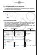
1-1 E-CON3 Application Overview 1 E-CON3 Application Overview This chapter describes the configuration of the E-CON3 application screen, and provides basic information about its menus and commands. Starting Up the E-CON3 Application u ClassPad Operation (1) Tap m on the icon panel to display the application menu. Next, swipe the screen to the left to display page two of the application menu. . (2) Tap This starts up the E-CON3 application and displays a Sensor Setup window.
1-2 E-CON3 Application Overview k Sensor Setup Window This window is for selecting a sensor for each of the Data Logger channels to be used for sampling, and for configuring sampling parameters. The Sensor Setup window has two tabs.
1-3 E-CON3 Application Overview E-CON3 Application Menus and Buttons This section provides an overview of E-CON3 application menu commands and toolbar buttons. k Menu Commands and Toolbar Buttons Common to All Windows Menu/Command Button O Variable Manager 5 View Window — Basic Format — Graph Format — Geometry Format — Advanced Format — Financial Format — Default Setup — Keyboard — Window Functions See the section about the O Menu in the ClassPad II User’s Guide.
1-4 E-CON3 Application Overview k Sensor Setup Window Menus Menu/Command Setup File Functions Displays the [Sample] tab of the Setup dialog box. The Setup dialog box has a [Sample] tab for advanced sampling parameters, a [Trigger] tab for advanced trigger parameters, and a [Graph] tab for graph settings. Open Setup Memory Recalls saved settings to the Sensor Setup window. Save Setup Memory Saves the settings on the Sensor Setup window under a file name for later recall.
1-5 E-CON3 Application Overview k E-CON Graph Window Menus and Buttons Menu/Command Zoom Button Functions All Zoom b Zooms all currently displayed graphs. Auto — Resizes the y-axis so the entire graph fits in the screen. The x-axis is adjusted automatically in accordance with the number of samples. y Auto R Resizes the graph so all of it fits in the screen along the y-axis, without changing the x-axis. Full — Resizes the graph so all of it fits in the screen.
1-6 E-CON3 Application Overview k E-CON Graph Window Menus and Buttons (Continued) Menu/Command Functions a Open Picture Fade I/O Saves the currently displayed graph as a graphic image (Save Picture). You can recall a saved graph image and overlay it on another graph to compare them (Open Picture). You can clear background image (Clear Picture). You can adjust the lightness of the background image (Fade I/O).
1-7 E-CON3 Application Overview E-CON3 Application Status Bar The following shows how the status bar appears for each of the E-CON3 application windows. k Sensor Setup Window Status Bar This item shows the currently selected sampling mode (Normal, Real-Time, Fast, Extended, or Period). For more information, see “Modes” on page 3-3. k E-CON Graph Editor Window Status Bar This item shows “Axes” when the E-CON Axes option is turned on, and nothing when E-CON Axes is turned off.
2-1 Basic Steps for Configuring Sampling Parameters 2 Basic Steps for Configuring Sampling Parameters This chapter explains the basic operations you need to perform when configuring Data Logger sampling parameters from the E-CON3 application. Before performing any of the procedures in this chapter, be sure to connect the Data Logger to your ClassPad. Configuring Parameters for Sampling with a Single Sensor Use the [Single] tab of the Sensor Setup window to configure the parameters for a single sensor.
2-2 Basic Steps for Configuring Sampling Parameters (2) Tap the [Sensor] box. • This displays a Select Sensor dialog box like the one shown to the right. (3) Select the sensor you will use for sampling. • Tap one of the tabs ([CMA], [CASIO], [Vernier], [Custom]), and then tap the option button next to the name of the sensor you want to select. For details about each of the selectable sensors, see the “10 Sensor List”.
2-3 Basic Steps for Configuring Sampling Parameters • Selecting some sensors will cause different parameters from those shown above to appear. The following table explains you should go for more information about such these sensors. For this type of sensor: Go here for more details: [CASIO] tab, [Microphone-FFT] See “Microphone-FFT Parameters” on page 2-4 for more information. [CMA] tab, [Photogate] or [Photogate (Pulley)] See “Photogate Sensor Parameters” on page 2-5 for more information.
2-4 Basic Steps for Configuring Sampling Parameters Tip • When you use the above procedure to configure sampling parameters for a single sensor, the sampling mode is selected automatically in accordance with the specified total sampling time. In this case, the parameters of the Setup dialog box’s [Sample] tab and [Trigger] tab are also configured automatically. The current sampling mode is indicated in the status bar.
2-5 Basic Steps for Configuring Sampling Parameters k Photogate Sensor Parameters Connection of a CMA or Vernier Photogate to the Data Logger requires configuration of parameters that are different from those for other types of sensors. u To configure a setup for Photogate alone In step (3) of the procedure under “To configure parameters for sampling with a single sensor” on page 2-1, select [Photogate] on the [CMA] or [Vernier] tab for the sensor.
2-6 Basic Steps for Configuring Sampling Parameters u To configure a setup for Photogate and Smart Pulley In step (3) of the procedure under “To configure parameters for sampling with a single sensor” on page 2-1, select [Photogate (Pulley)] on the [CMA] or [Vernier] tab for the sensor. This causes the parameters described below to appear on the Sensor Setup window that appears in step (4).
2-7 Basic Steps for Configuring Sampling Parameters Configuring Parameters for Sampling with Multiple Sensors Use the [Multiple] tab to configure parameters for simultaneous sampling with multiple sensors. The [Multiple] tab lets you select up to three channels for sampling, from among the Data Logger’s CH1, CH2, CH3, and SONIC* channels. * EA-200 only u To configure parameters for sampling with multiple sensors (1) Start up the E-CON3 application.
2-8 Basic Steps for Configuring Sampling Parameters (4) Select the sensors you will use for sampling. • Depending on the sensors you have connected to each channel, select the [CMA], [CASIO], [Vernier], or [Custom] tab and then tap the option button for the applicable sensor name. For details about the sensors that can be selected for each channel, see the “10 Sensor List”. • Tapping the [Custom] tab displays a sheet for configuring the parameters of a userdefined custom probe.
2-9 Basic Steps for Configuring Sampling Parameters (9) Use the [Sample] and [Trigger] tabs of the Setup dialog box to configure the required parameters. • For details about the required parameters in each mode, see “Mode Parameters” on page 3-5. (10) To apply the current settings on the Setup dialog box, tap [Set]. • This closes the Setup dialog box. (11) You can start sampling immediately or you can save the setup in memory for later recall. • To start sampling immediately, tap S.
3-1 Setup 3 Setup This chapter explains the various parameters you can configure with the Setup dialog box. Important! • Configuring advanced setup parameters is optional in the case of single-sensor sampling. See “To configure advanced parameters for a single sensor” on page 3-2. • With multiple-sensor sampling, advanced setup parameters are part of the normal configuration procedure. See steps (7) through (10) under “To configure parameters for sampling with multiple sensors” on page 2-7.
3-2 Setup Configuring Advanced Sampling Parameters This section explains how to configure advanced sampling parameters on the [Sample] and [Trigger] tabs of the Setup dialog box. u To configure advanced parameters for a single sensor (1) Perform steps (1) through (6) under “To configure parameters for sampling with a single sensor” on page 2-1. (2) On the menu bar, tap [Setup]. • This displays the [Sample] tab of the Setup dialog box.
3-3 Setup (6) You can now start sampling immediately or you can save the setup in memory for later recall. • To start sampling immediately, tap S. See “5 Executing a Sampling Operation” for more information. • To store the setup in memory, tap [File] on the menu bar, and then tap [Save Setup Memory]. See “4 Using Setup Memory” for more information. Modes The [Mode] box at the top of the [Sample] tab of the Setup dialog box controls the current mode setting.
3-4 Setup k Extended Mode The Extended Mode is the opposite of the Fast Mode in that it allows setting of a long sampling interval. In this mode, the sampling interval can be set in a range of 5 to 240 minutes. This mode is best for sampling data like temperature or humidity over a long period. While performing measurements with the Extended mode, the Data Logger will enter a power off sleep state while standing by.
3-5 Setup Mode Parameters This section explains the parameters that can be configured on the [Sample] tab and [Trigger] tab of the Setup dialog box, in accordance with the mode selected on the [Sample] tab. k Parameters Common to All Modes The following explains the parameters that normally appear, regardless of the currently selected mode. Sampling Interval: Specify a value for the sampling interval. If you specify an interval of one second, for example, a sample will be taken every second.
3-6 Setup k Normal Mode Parameters Tab [Sample] [Trigger] Parameter Sampling Interval Initial Default 0.05 sec Range 0.0005 to 299 sec* Number of Samples 100 10 to 30000 Warm-Up Auto Auto, Manual (1 to 999) Start Trigger Tap Screen Tap Screen, Count Down, CH1, SONIC, Microphone * When one of the motion sensors is selected for the sensor, the setting range becomes 0.02 to 299 seconds. • For details about each parameter, see “Parameters Common to All Modes” on page 3-5.
3-7 Setup FFT Graph The [FFT Graph] parameter is available only when [Microphone] is selected as the sensor. You can turn post-sampling FFT Graph (frequency characteristics graph) graphing on or off. When [CASIO] - [Microphone] is the sensor: In this case, the initial setting for the FFT graph is off. Turning on the FFT graph causes [Frequency Pitch] and [Frequency Max] values to be calculated. Note that these calculated values area applied automatically, and cannot be changed.
3-8 Setup Number of Samples: Specify the number of samples that should be collected. Sampling continues until the specified number of samples is collected, regardless of the sampling time. Warm-Up: See “Parameters Common to All Modes” on page 3-5. Start Trigger: CH1 is always the start trigger. Sampling is triggered in accordance with the input value of the sensor connected to the CH1 channel. The timing of the trigger is controlled in accordance with the following two parameters.
3-9 Setup k Additional Start Trigger Parameters The following are the parameters that need to be configured for the Count Down, CH1, SONIC, and Microphone start triggers when Normal, Real-Time, or Fast is selected as the mode. • If you specify CH1, SONIC, or Microphone for the [Start Trigger] parameter, you should also use the [Trigger] tab of the Setup dialog box to specify an appropriate start trigger for the selected sensor.
3-10 Setup The graphs below show when sampling is triggered while [Rising] is specified for [Trigger Edge]. The graphs show changes in sampled values over time, and the left end of the graph is when the sampling operation is executed.
3-11 Setup The graphs below show when sampling is triggered while [Above] is specified for [Trigger Level]. The graphs show changes in sampled values over time, and the left end of the graph is when the sampling operation is executed. Threshold value Sampling triggered Sampling triggered Microphone Start Trigger Additional Parameter Sensitivity Initial Default High Range Low, Medium, High Sensitivity: Specify one of three sensitivity levels for the EA-200’s microphone.
3-12 Setup k Graph Options The following provides detailed explanations of the options that are available on the [Graph] tab of the Setup dialog box. Option Description Initial Default Setting Graph Function Turns display of the source data name (current data channel name or sampling memory data name) on the E-CON Graph window on (selected) and off (cleared).
3-13 Setup (4) When the name is the way you want, tap [OK]. • This displays the Custom Probe dialog box. (5) Configure the following parameters on the Custom Probe dialog box. Parameter Description Slope Input the slope for the linear interpolation formula. Intercept Input the intercept for the linear interpolation formula. Unit Name Input up to eight characters for the unit name. Warm-Up Specify the warm-up time for the sensor in seconds, from 0 to 999.
3-14 Setup u To edit an existing custom probe (1) On the Sensor Setup window, make sure that the custom probe you want to edit is not selected. • If the name of the custom probe you want to edit is displayed in the [Sensor] box on the [Single] tab of the Sensor Setup window, or in the [CH1], [CH2], [CH3], or [SONIC] box of the [Multiple] tab, tap the applicable box and then change its setting to something other than the probe you want to edit.
3-15 Setup u To configure new custom probe settings based on CMA or Vernier sensor settings Use the following procedure to recall CMA or Vernier sensor settings that you have already registered with the E-CON3 application and use them to configure a new custom probe. (1) On the Sensor Setup window [Tool] menu, tap [Custom Probe] and then tap [Edit CMA Sensor] or [Edit Vernier Sensor]. • This displays the Select Sensor dialog box.
3-16 Setup u To calibrate a custom probe Note • Perform the following procedure to calibrate a custom probe after you newly configure it or after you edit its settings. • This procedure calibrates slope and intercept values based on two actual samples using the applicable custom probe. • Before performing the procedure below, you should prepare two conditions whose measurement values are known.
3-17 Setup (5) In the [Value 1] box, input the reference value for the first sample, and then tap [OK]. • This restarts sampling by the sensor connected to the CH1 channel and displays a Sampling... dialog box like the one shown to the right. This is how the dialog box appears during standby prior to the second sample. • If this dialog box is left on the display, sampling will terminate and the dialog box will close automatically after about five hours.
3-18 Setup u To zero adjust a custom probe This procedure zero adjusts a custom probe and sets its intercept value based on an actual sample using the applicable custom probe. (1) Connect the Data Logger to your ClassPad, and connect the custom probe you want to zero adjust to the Data Logger’s CH1 channel. (2) What you should do next depends on whether you are calibrating a new custom probe or an existing custom probe whose settings have been edited.
4-1 Using Setup Memory 4 Using Setup Memory Setup memory lets you save the parameters on the Sensor Setup window in a file for later recall when you need them. This means you can instantly setup for a particular sensor simply by recalling a setup. Setup Memory Data File Contents Saving Sensor Setup window parameters saves the following data in setup memory.
4-2 Using Setup Memory u To recall setup data Important! • Performing the following procedure will replace the current settings of the Sensor Setup window parameters (see “Setup Memory Data File Contents” on page 4-1) with the setup data you recall. (1) Display the Sensor Setup window active. • It makes no difference whether the [Single] tab or [Multiple] tab is displayed. (2) On the [File] menu, tap [Open Setup Memory]. • This displays the Open Data dialog box.
5-1 Executing a Sampling Operation 5 Executing a Sampling Operation This chapter explains the procedure for executing a Data Logger sampling operation in accordance with E-CON3 application settings. It also explains how to store sample data collected with the Data Logger. Note (EA-200 only) • For information about operation when [CASIO] - [Speaker ( y = f (x))] is selected as the sensor on the Sensor Setup window, see “6 Outputting a Function to the Speaker”.
5-2 Executing a Sampling Operation (3) Depending on the setup you are using, either a standby dialog box appears or sampling starts right away after configuration of the Data Logger settings is complete. • What happens next depends on the sampling mode, trigger settings, and other setup data sent to the Data Logger. For details, see “Operations Performed during Sampling” below. • After sampling is complete, the sampled data is stored temporarily as “current data”.
3HULRG ([WHQGHG 5HDO 7LPH 0RGH 6WDUW 6WDQGE\ &DQFHOV VDPSOLQJ DQG GLVFDUGV VDPSOHG GDWD 7KH JUDSK LV GUDZQ XVLQJ WKH GDWD IURP WKH EHJLQQLQJ RI WKH VDPSOLQJ RSHUDWLRQ XS WR WKH SUHVHQW 'DWD LV JUDSKHG LQ UHDO WLPH DV LW LV VDPSOHG 6DPSOLQJ RSHUDWLRQ LV WULJJHUHG DQG GDWD LV JUDSKHG 6DPSOLQJ HQGV This dialog box appears when sampling is finished. Sampled data is stored in a specified memory area, and can be viewed with the Main application or Stat Editor.
1RUPDO )DVW 0RGH 6WDUW 6WDQGE\ 7KH VFUHHQ VKRZQ EHORZ DSSHDUV ZKHQ &+ 621,& RU 0LFURSKRQH LV XVHG DV WKH 6WDUW 7ULJJHU 7KH HODSVHG VDPSOLQJ WLPH LV FRXQWHG RQ WKH GLVSOD\ GXULQJ VDPSOLQJ &DQFHOV VDPSOLQJ DQG GLVFDUGV VDPSOHG GDWD 6DPSOLQJ RSHUDWLRQ LV WULJJHUHG DQG GDWD LV JUDSKHG 1RUPDO 0RGH JUDSKLQJ H[DPSOH )DVW 0RGH JUDSKLQJ H[DPSOH 6DPSOLQJ HQGV DQG GDWD LV JUDSKHG 5-4 Executing a Sampling Operation
5-5 Executing a Sampling Operation Saving Sample Data The data produced by a Data Logger sampling operation controlled from the E-CON3 application is stored temporarily in the ClassPad’s [EConSamp] folder. This temporary data is called the “current data”. • Current data is saved using one or more variables, one for each of the channels that was used for sampling. Variable names are assigned automatically in accordance with the channel and sensor used for sampling.
5-6 Executing a Sampling Operation You can use the [Current] tab to graph the current data after sampling is complete. For information about graphing, see “8 Graphing Data”. • Whenever you perform a new sampling operation, the current data of the channel you are using is overwritten with the new data. If you want to keep a copy of sampled data, you need to save the current data under a different name.
6-1 Outputting a Function to the Speaker 6 Outputting a Function to the Speaker (EA-200 only) When [Speaker (y = f(x))] is selected on the [CASIO] tab of the Select Sensor dialog box, sampling is not performed by a sensor. Instead, the sound of the waveform of a function input on the ClassPad is output from the EA-200’s speaker. u To output the waveform of a function through the speaker (1) Connect the EA-200 to the ClassPad, and turn on the EA-200.
6-2 Outputting a Function to the Speaker • When [Manual] is selected, the optimization performed by the [Auto] setting is not performed. Because of this, you need to input a function and specify an output range (x-value) that makes the y-axis range –1.5 to 1.5. An error occurs whenever the y-axis is outside the range of –1.5 to 1.5. (9) Tap the [Formula] down arrow button. On the menu that appears, select the line ( y1 to y20) that contains the function you input in step (4).
7-1 Using the Multimeter Window 7 Using the Multimeter Window The Multimeter window shows the sample values of all channels in real-time. You can also use the Multimeter window to manually store sample data at any point. Viewing Sample Data on the Multimeter Window This section explains how to view sample data in real-time on the Multimeter window. Tip • Before performing the procedures described here, perform the preparation steps under “To get ready for sampling” on page 5-1.
7-2 Using the Multimeter Window u To view real-time sample data during sampling configured with the [Single] tab (1) On the Sensor Setup window, display the [Single] tab and configure the settings you want. • You can also recall previously saved setup data (page 4-2). (2) Tap /. • This displays the Multimeter window and starts sampling with the sensor connected to the channel specified on the [Single] tab. Sampled data is displayed in real-time on the Multimeter window.
7-3 Using the Multimeter Window u To view real-time sample data during sampling configured with the [Multiple] tab (1) On the Sensor Setup window, display the [Multiple] tab and configure the settings you want. • You can also recall previously saved setup data (page 4-2). (2) Tap /. • This displays the Multimeter window and starts sampling with the sensors connected to the channels specified on the [Multiple] tab. Sampled data is displayed in real-time on the Multimeter window.
7-4 Using the Multimeter Window Saving Sample Data from the Multimeter Window You can use the procedures below to save sample data while the Multimeter window is displayed. Executing sample data save from the Multimeter window saves the current sample data only. u To save sample data from the Multimeter window during sampling configured with the [Single] tab (1) Perform steps (1) and (2) of the procedure under “To view real-time sample data during sampling configured with the [Single] tab” on page 7-2.
7-5 Using the Multimeter Window u To save sample data from the Multimeter window during sampling configured with the [Multiple] tab (1) Perform steps (1) and (2) of the procedure under “To view real-time sample data during sampling configured with the [Multiple] tab” on page 7-3. (2) When you want to store sample data, tap the [Save] button on the Multimeter window. • This causes the count value on the window to change from 0 to 1.
8-1 Graphing Data 8 Graphing Data This chapter explains how to configure graph parameters on the E-CON Graph Editor window, and how to draw a graph on the E-CON Graph window. E-CON Graph Editor Window To graph sample data, you first need to tap the c button and display the E-CON Graph Editor window, where you can select the sample data you want to graph. The E-CON Graph Editor window has three tabs: [Current], [Normal], and [Compare]. Each of the tabs is described in detail below.
8-2 Graphing Data Upper/Lower Style This is the same style as the [Compare] tab (see page 8-4). This style appears in the following cases only. • When sampling is performed with [CASIO] - [Speaker (Sample Data)] specified as the sensor • When sampling is performed with [CASIO]- [Microphone] specified as the sensor, with the [FFT Graph] setting turned on. • When sampling is performed with [Vernier]-[Microphone] specified as the sensor, with the [FFT Graph] setting turned on.
8-3 Graphing Data k [Normal] Tab The [Normal] tab is for recalling previously saved sampled data (or current data) for graphing. You can draw up to three graphs at the same time using this tab. Graphs You can draw the following types of graphs using the [Normal] tab. • Different sampled data can be recalled and assigned to each of the graphs (Gph1, Gph2, Gph3) and graphed at the same time. • You can use this tab to draw a single graph, or to draw two or three graphs at the same time.
8-4 Graphing Data k [Compare] Tab Like the [Normal] tab, the [Compare] tab lets you for recall previously saved sampled data (or current data) for graphing. You can draw up to two graphs at the same time using this tab. Graphs You can draw the following types of graphs using the [Compare] tab. • Different sampled data can be recalled and assigned to each of the graphs (Upper and Lower) and graphed at the same time. • You can use this tab to draw a single graph or to draw two graphs at the same time.
8-5 Graphing Data Drawing a Graph The following procedures explain how to actually draw a graph by configuring setups on each of the E-CON Graph Editor window tabs. u To draw a graph using [Normal] tab settings (1) Tap c to display the E-CON Graph Editor window. (2) Tap the [Normal] tab. (3) First, recall the data you want to assign to [Gph1]. Tap the [Gph1] box. Tap here. • This displays a Open Data dialog box like the one shown below. (4) Tap the [Folder] option button.
8-6 Graphing Data (8) Assign sample data to [Gph2] and [Gph3]. • If you want to recall and assign different data, repeat steps (3) through (7) above for [Gph2] and/or [Gph3]. • If you want to perform first derivative or second derivative on [Gph1] and assign the results to [Gph2] or [Gph3], perform the following steps. Note, however, that you will be able to perform these steps only if you have data assigned to [Gph1].
8-7 Graphing Data (12) Tapping the [xyLine] or [Scatter] down arrow button displays a list of the plot point types. • The following shows the type of graph produced by each possible setting available on the Graph Plot Type dialog box. xyLine Scatter dot large dot square cross (13) Tap [Set]. • This closes the Graph Plot Type dialog box. The current plots settings are indicated under each of the graph names (Gph1, Gph2, Gph3) on the E-CON Graph Editor window.
8-8 Graphing Data u To draw a graph using [Compare] tab settings (1) Tap c to display the E-CON Graph Editor window. (2) Tap the [Compare] tab. (3) First, recall the data you want to assign to [Upper]. Tap the [Upper] box. Tap here. • This displays a Open Data dialog box like the one shown below. (4) Tap the [Folder] option button. (5) Tap the [Folder] down arrow button, and then tap the name of folder that contains the sample you want to recall.
8-9 Graphing Data (8) Assign sample data to [Lower]. • If you want to recall and assign different data, repeat steps (3) through (7) above for [Lower]. • If you want to assign [Upper] first derivative data or second derivative data, or [Upper] data converted to a format for output through the speaker, perform the following steps. Note, however, that you will be able to perform these steps only if you have data assigned to [Upper].
8-10 Graphing Data u To draw a graph using [Current] tab settings • In either of the following cases, perform the same steps as those under “To draw a graph using [Compare] tab settings” on page 8-8. • When sampling is performed with [CASIO] - [Speaker (Sample Data)] specified as the sensor • When sampling is performed with [CASIO] - [Microphone] specified as the sensor, with the [FFT Graph] setting turned on.
9-1 E-CON Graph Window Operations 9 E-CON Graph Window Operations This chapter explains how to perform zoom, scroll, and other operations while a graph is on the E-CON Graph window. It also explains how to use various analytical tools. Note The E-CON Graph window appears and a data is graphed after either of the following two events.
9-2 E-CON Graph Window Operations (4) To exit the zoom mode, tap l on the ClassPad icon panel, or press the ClassPad c key. u To zoom a particular graph Note • Use this procedure to zoom a particular graph while there are multiple graphs on the E-CON Graph window. • You will not be able to zoom a graph drawn by assigning data to [Gph2], [Gph3], or [Lower] with the [Special] option on the Open Data dialog box. See pages 8-6 and 8-9 for more information. (1) On the E-CON Graph window a menu tap [1Zoom].
9-3 E-CON Graph Window Operations Displaying and Hiding Graph Display Components When there are multiple graphs on the E-CON Graph window, you can display or hide the graph axes, the source data name, and the axis labels. u To hide and display the source data name and axes When you have multiple graphs on the display, the source data name and axes of the first graph appear first.
9-4 E-CON Graph Window Operations Scrolling a Graph You can select one of the graphs displayed on the E-CON Graph window and scroll it. • Note that you will not be able to scroll a graph drawn by assigning data to [Gph2], [Gph3], or [Lower] with the [Special] option on the Open Data dialog box. See pages 8-6 and 8-9 for more information. u To scroll a particular graph (1) On the E-CON Graph window a menu, tap [1Move].
9-5 E-CON Graph Window Operations Using Trace Trace displays a cross pointer on the displayed graph along with the coordinates of the current cursor position. You can use the cursor keys to move the pointer along the graph. • Note that you will not be able to perform the trace operation cannot on a graph drawn by assigning data to [Gph2], [Gph3], or [Lower] with the [Special] option on the Open Data dialog box. See pages 8-6 and 8-9 for more information.
9-6 E-CON Graph Window Operations Calculating the Periodic Frequency You can use the following procedure to determine the periodic frequency for a specific range on a graph. • Note that you will not be able to calculate the periodic frequency for a graph drawn by assigning data to [Gph2], [Gph3], or [Lower] with the [Special] option on the Open Data dialog box. See pages 8-6 and 8-9 for more information.
9-7 E-CON Graph Window Operations Analyzing a Graph Using Fourier Series Expansion Fourier series expansion is effective for studying sounds by expressing them as functions. The procedure below assumes that there is a graph of sampled sound data already on the graph screen. • Fourier series expansion is possible only with data sampled using the EA-200’s built-in microphone. Attempting the following procedure with any other type of data causes an error.
9-8 E-CON Graph Window Operations (4) On the dialog box, configure the settings as required. Parameter Description Graph Sheet Specify a Graph Editor window sheet from Sheet 1 to Sheet 5 for storage of the numeric expression that results from Fourier series expansion. Note that any function expressions input on the sheet you specify here are overwritten. Start Specify a value from 1 to 99 for the Fourier series expansion start degree.
9-9 E-CON Graph Window Operations (5) After all the settings are the way you want, tap [OK]. • This starts calculation. The Graph Editor window containing the numeric expression obtained as a result of the Fourier series expansion appears in the lower half of the screen when calculation is complete. At this time, the Graph Editor window is active. (6) On the toolbar, tap $ to graph the expression obtained as the result of the Fourier series expansion on the Graph window.
9-10 E-CON Graph Window Operations (3) On the Save Data dialog box, specify the name of the folder where the list variable is stored and the list name. • Time and data are stored in different lists. Specify a list name for each. • The time value is always stored as seconds. Tap here and then select the destination folder from the list that appears. Use the keyboard to input the variable name. (4) After the settings are configured in the way you want, tap [OK].
9-11 E-CON Graph Window Operations Tip • Note that you will not be able to save data of a graph drawn by assigning data to [Gph2], [Gph3], or [Lower] with the [Special] option on the Open Data dialog box. See pages 8-6 and 8-9 for more information. u To save all of a graph’s data to a matrix type variable (1) On the E-CON Graph window [File] menu, tap [Save Matrix] and then [All]. • This displays the Save Data dialog box.
9-12 E-CON Graph Window Operations u Saved Matrix Data Saving graph data to a matrix type variable saves it to a variable that has n lines and up to 6 columns, where n is the total number of samples in the saved data. • If the maximum number of graphs are not on the display (less than three in the case of Gph1, Gph2, Gph3; less than 2 in the case of Upper and Lower), data is not saved for the unused graph(s).
9-13 E-CON Graph Window Operations Outputting a Graph as a Sound from the Speaker (EA-200 only) You can specify a range on a graph and output it from the speaker. Note • The following operation is possible only with data sampled using the EA-200’s built-in microphone. Attempting the following procedure with any other type of data, including that sampled with [CASIO] - [Microphone-FFT] causes an error. The allowable output range is 200 to 4000 Hz.
9-14 E-CON Graph Window Operations (7) Tap [OK]. • This outputs the waveform between the start point and end point from the EA-200’s speaker. • An error will result if the sound you configured cannot be output for some reason. Note that the supported output range is 200 to 4000 Hz. If an error occurs, tap [OK] and then perform the procedure from the beginning. (8) To terminate sound output, press the EA-200 [START/STOP] key.
9-15 E-CON Graph Window Operations (4) After the settings are configured is the way you want, tap [OK]. • This displays a dialog box like the one shown to the right. (5) Tap [OK]. • This outputs the sampled sound from the EA-200’s speaker. (6) To terminate sound output, press the EA-200 [START/STOP] key. (7) Tap [OK]. This returns to the Speaker Output window of step (1). • To return to the E-CON Graph window, tap the [Stop] button.
9-16 E-CON Graph Window Operations Tip • The time value is always stored as seconds. • The storage capacity of the above data storage operation is limited. If an error occurs, use [File] [Save List] to store the data as a list.
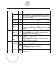
10-1 Sensor List 10 Sensor List The following is a list of sensors that can be selected on the Sensor Setup window. The “䊊” symbol indicates sensors that can be selected for the applicable tab ([Single] or [Multiple]) and channel.
10-2 Sensor List Manufacturer CMA* 1 Sensor Name [Multiple] Tab CH1 CH1, CH2, CH3 Force ±50 (N) 䊊 䊊 Force Plate 800 (N) 䊊 䊊 Force Plate 3500 (N) 䊊 䊊 Gas Pressure (kPa) 䊊 䊊 Heart Rate (%) 䊊 䊊 2 Light 10 (W/m ) 䊊 䊊 Light 10 (lx) 䊊 䊊 Light 200 (lx) 䊊 䊊 Light 150 (klx) 䊊 䊊 Magnetic Field 50 (mT) 䊊 䊊 Magnetic Field 500 (mT) 䊊 䊊 ORP (mV) 䊊 䊊 Oxygen Gas (%) 䊊 䊊 pH (pH) 䊊 䊊 Photogate 䊊 Photogate (Pulley) 䊊 Pressure 023i (kPa) 䊊 䊊 Pressure BT66i 130 (kPa) 䊊
10-3 Sensor List Manufacturer CASIO Vernier*4 Sensor Name [Single] Tab CH1 [Multiple] Tab CH1, CH2, CH3 Microphone * Microphone-FFT *2 Speaker (Sample Data) *2 Speaker (y = f(x)) *3 Low-g Accel H (m/s2) 䊊 䊊 Low-g Accel V (m/s2) 䊊 䊊 25-g Accel H (m/s2) 䊊 䊊 25-g Accel V (m/s ) 䊊 䊊 Barometer (atm) 䊊 䊊 Barometer (inHg) 䊊 䊊 Barometer (mbar) 䊊 䊊 Barometer (mmHg) 䊊 䊊 Conductivity 100 (mg/L) 䊊 䊊 Conductivity 1000 (mg/L) 䊊 䊊 Conductivity 10000 (mg/L) 䊊 䊊 Conductivity 20
10-4 Sensor List Manufacturer Vernier Custom *1 *2 *3 *4 Sensor Name [Single] Tab CH1 Photogate 䊊(SONIC) Photogate (Pulley) 䊊(SONIC) [Multiple] Tab CH1, CH2, CH3 pH (pH) 䊊 䊊 Pressure (atm) 䊊 䊊 Pressure (kPa) 䊊 䊊 Pressure (mmHg) 䊊 䊊 Pressure (psi) 䊊 䊊 Thermocouple (°C) 䊊 䊊 User-assigned name and unit 䊊 䊊 SONIC Centre for Microcomputer Applications EA-200 built-in microphone used as sensor. Sound output from EA-200 built-in speaker in accordance with specified function.
CASIO COMPUTER CO., LTD. 6-2, Hon-machi 1-chome Shibuya-ku, Tokyo 151-8543, Japan SA1605-A © 2016 CASIO COMPUTER CO., LTD.