EN fx-CG50 (Version 3.60) fx-CG50 AU (Version 3.60) fx-CG20 (Version 3.12) fx-CG20 AU (Version 3.12) fx-CG10 (Version 3.12) Software User’s Guide CASIO Worldwide Education Website https://edu.casio.com Manuals are available in multi languages at https://world.casio.
• The contents of this user’s guide are subject to change without notice. • No part of this user’s guide may be reproduced in any form without the express written consent of the manufacturer. • Be sure to keep all user documentation handy for future reference.
Contents Getting Acquainted — Read This First! Chapter 1 Basic Operation 1. 2. 3. 4. 5. 6. 7. 8. 9. 10. Keys .............................................................................................................................. 1-1 Display .......................................................................................................................... 1-3 Inputting and Editing Calculations .................................................................................
12. Drawing Dots, Lines, and Text on the Graph Screen (Sketch) ................................... 5-52 13. Function Analysis ........................................................................................................ 5-54 Chapter 6 Statistical Graphs and Calculations 1. 2. 3. 4. 5. 6. 7. 8. 9. Before Performing Statistical Calculations .................................................................... 6-1 Calculating and Graphing Single-Variable Statistical Data ...........................
Chapter 11 Memory Manager 1. Using the Memory Manager ........................................................................................ 11-1 Chapter 12 System Manager 1. Using the System Manager ......................................................................................... 12-1 2. System Settings .......................................................................................................... 12-1 Chapter 13 Data Communication 1.
Appendix 1. Error Message Table ....................................................................................................α-1 2. Input Ranges ..............................................................................................................α-14 Examination Modes ..................................................................................... β-1 E-CON4 Application 1. 2. 3. 4. 5. 6. 7. 8. 9. 10. 11. 12. 13. E-CON4 Mode Overview.....................................................
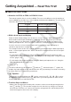
Getting Acquainted — Read This First! k About this User’s Guide u Attention fx-CG10, fx-CG20, fx-CG20 AU Users This manual explains how to use the fx-CG50. There are some differences in the marking of some fx-CG50 keys and the keys of the fx-CG10, fx-CG20, and fx-CG20 AU. The table below shows the differences in key markings.
• This User’s Guide shows the current operation assigned to a function key in parentheses following the key cap for that key. 1(Comp), for example, indicates that pressing 1 selects {Comp}, which is also indicated in the function menu. • When (g) is indicated in the function menu for key 6, it means that pressing 6 displays the next page or previous page of menu options. u Menu Titles • Menu titles in this User’s Guide include the key operation required to display the menu being explained.
Chapter 1 Basic Operation 1.
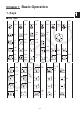
k Key Markings Many of the calculator’s keys are used to perform more than one function. The functions marked on the keyboard are color coded to help you find the one you need quickly and easily. Function Key Operation 1 log l 2 10x !l 3 B al The following describes the color coding used for key markings. Color • Key Operation Yellow Press ! and then the key to perform the marked function. Red Press a and then the key to perform the marked function.
2. Display k Selecting Icons This section describes how to select an icon in the Main Menu to enter the mode you want. u To select an icon 1. Press m to display the Main Menu. 2. Use the cursor keys (d, e, f, c) to move the highlighting to the icon you want. Currently selected icon 3. Press w to display the initial screen of the mode whose icon you selected.
Icon Mode Name Description Recursion Use this mode to store recursion formulas, to generate a numeric table of different solutions as the values assigned to variables in a function change, and to draw graphs. Conic Graphs Use this mode to draw graphs of conic sections. Equation Use this mode to solve linear equations with two through six unknowns, and high-order equations from 2nd to 6th degree. Program Use this mode to store programs in the program area and to run programs.
k About the Function Menu Use the function keys (1 to 6) to access the menus and commands in the menu bar along the bottom of the display screen. You can tell whether a menu bar item is a menu or a command by its appearance. k Status Bar The status bar is an area that displays messages and the current status of the calculator. It is always displayed at the top of the screen. • Icons are used to indicate the information described below. This icon: Indicates this: The current battery level.
k About Display Screens This calculator uses two types of display screens: a text screen and a graph screen. The text screen can show 21 columns and 8 lines of characters, with the bottom line used for the function key menu. The graph screen uses an area that measures 384 (W) × 216 (H) dots. Text Screen Graph Screen k Normal Display The calculator normally displays values up to 10 digits long. Values that exceed this limit are automatically converted to and displayed in exponential format.
k Special Display Formats This calculator uses special display formats to indicate fractions, hexadecimal values, and degrees/minutes/seconds values. u Fractions .................... Indicates: 456 12 23 u Hexadecimal Values .................... Indicates: 0ABCDEF1(16), which equals 180150001(10) u Degrees/Minutes/Seconds .................... Indicates: 12° 34’ 56.
u To change a step Example To change cos60 to sin60 Acga ddd D s u To delete a step Example To change 369 × × 2 to 369 × 2 Adgj**c dD In the insert mode, the D key operates as a backspace key. u To insert a step Example To change 2.362 to sin2.362 Ac.dgx ddddddd s k Parentheses Colors during Calculation Formula Input Parentheses are color coded during input and editing of calculation formulas in order to make it easier to confirm the proper relationship between opening and closing parentheses.
• Inputting a closing parenthesis assigns it the same color as the corresponding opening parenthesis. • The parentheses of parenthetical expressions that are of the same level are the same color. Executing a calculation causes the color of all parentheses to become black. k Using Replay Memory The last calculation performed is always stored into replay memory. You can recall the contents of the replay memory by pressing d or e. If you press e, the calculation appears with the cursor at the beginning.
After you press A, you can press f or c to recall previous calculations, in sequence from the newest to the oldest (Multi-Replay Function). Once you recall a calculation, you can use e and d to move the cursor around the calculation and make changes in it to create a new calculation. Example 2 Abcd+efgw cde-fghw A f (One calculation back) f (Two calculations back) • A calculation remains stored in replay memory until you perform another calculation.
k Using the Clipboard for Copy and Paste You can copy (or cut) a function, command, or other input to the clipboard, and then paste the clipboard contents at another location. Note In the Math input/output mode, the copy (or cut) range you can specify is limited by the range of movement of the cursor. In the case of parentheses, you can select any range within a parenthetical expression or you can select the entire parenthetical expression. u To specify the copy range 1.
u Pasting Text Move the cursor to the location where you want to paste the text, and then press !j(PASTE). The contents of the clipboard are pasted at the cursor position. A !j(PASTE) k Catalog Function The Catalog is a list of all the commands available on this calculator (except for Python mode). You can input a command by displaying the catalog screen and then selecting the desired command. • Commands are divided into categories.
Example: To input the “FMax(” command, which determines a maximum value A!e(CATALOG)6(CAT) c1(EXE) cc1(EXE) cccccc 1(INPUT) To close the catalog screen, press J or !J(QUIT). u Searching for a Command This method is helpful when you know the name of the command you want to input. 1. Press !e(CATALOG) to display the catalog screen. 2. Press 6(CAT) to display the category list. 3. Move the highlighting to “1:ALL” and then press 1(EXE) or w. • This displays a list all the commands. 4.
Example: To input the command “FMax(” A!e(CATALOG)6(CAT) 1(EXE)t(F)h(M) 1(INPUT) u Using the Command History The calculator maintains a history of the last six commands you input. 1. Display one of the command lists. 2. Press 5(HISTORY). • This displays the command history. 3. Use f and c to move the highlighting to the command you want to input and then press 1(INPUT) or w. u QR Code Function • You can use the QR Code function to access the online manual that covers commands.
1. Select a command that is included in the online manual. • This causes 2(QR) to appear in the function menu. 2. Press 2(QR). • This displays a QR Code. 3. Use your smart device to read the displayed QR Code. • This will display the online manual on your smart device. • For information about how to read a QR Code, refer to the user documentation of your smart device and the QR Code reader you are using. • If you are having trouble reading the QR Code, use d and e to adjust display brightness. 4.
k Input Operations in the Math Input/Output Mode u Math Input/Output Mode Functions and Symbols The functions and symbols listed below can be used for natural input in the Math input/output mode. The “Bytes” column shows the number of bytes of memory that are used up by input in the Math input/output mode.
u Using the MATH Menu In the Run-Matrix mode, pressing 4(MATH) displays the MATH menu. You can use this menu for natural input of matrices, derivatives, integrals, etc. • {MAT/VCT} ... displays the MAT/VCT submenu, for natural input of matrices/vectors • {2×2} ... inputs a 2 × 2 matrix • {3×3} ... inputs a 3 × 3 matrix • {m×n} ... inputs a matrix/vector with m lines and n columns (up to 6 × 6) • {2×1} ... inputs a 2 × 1 vector • {3×1} ... inputs a 3 × 1 vector • {1×2} ... inputs a 1 × 2 vector • {1×3} ...
Example 2 ( To input 1+ 2 5 ) 2 A(b+ ' cc f e )x w 1 Example 3 To input 1+ 0 x + 1dx Ab+4(MATH)6(g)1(∫dx) v+b ea fb e w 1-18
Example 4 To input 2 × 1 2 2 2 1 2 Ac*4(MATH)1(MAT/VCT)1(2×2) 'bcc ee !x(')ce e!x(')cee'bcc w u When the calculation does not fit within the display window Arrows appear at the left, right, top, or bottom edge of the display to let you know when there is more of the calculation off the screen in the corresponding direction. When you see an arrow, you can use the cursor keys to scroll the screen contents and view the part you want.
u Math Input/Output Mode Input Restrictions Certain types of expressions can cause the vertical width of a calculation formula to be greater than one display line. The maximum allowable vertical width of a calculation formula is about two display screens. You cannot input any expression that exceeds this limitation. u Using Values and Expressions as Arguments A value or an expression that you have already input can be used as the argument of a function.
This capability can be used with the following functions.
• Note the following cursor operations you can use while inputting a calculation with Math input/output mode.
k Math Input/Output Mode Calculation Result Display Fractions, matrices, vectors, and lists produced by Math input/output mode calculations are displayed in natural format, just as they appear in your textbook. Sample Calculation Result Displays • Fractions are displayed either as improper fractions or mixed fractions, depending on the “Frac Result” setting on the Setup screen. For details, see “Using the Setup Screen” (page 1-35). • Matrices are displayed in natural format, up to 6 × 6.
k History Function The history function maintains a history of calculation expressions and results in the Math input/output mode. Up to 30 sets of calculation expressions and results are maintained. b+cw *cw You can also edit the calculation expressions that are maintained by the history function and recalculate. This will recalculate all of the expressions starting from the edited expression.
k Calculation Operations in the Math Input/Output Mode This section introduces Math input/output mode calculation examples. • For details about calculation operations, see “Chapter 2 Manual Calculations”. u Performing Function Calculations Using Math Input/Output Mode Example Operation 6 = 3 4 × 5 10 A6'4*5w cos π = 1 (Angle: Rad) 3 2 Ac(!5(π)'3e)w log28 = 3 A4(MATH)2(logab) 2e8w 7 A!M(x') 7e123w ( ) 123 = 1.988647795 2 + 3 × 3 64 − 4 = 10 log 3 = 0.
k Performing Matrix/Vector Calculations Using Math Input/Output Mode u To specify the dimensions (size) of a matrix/vector 1. In the Run-Matrix mode, press !m(SET UP)1(Math)J. 2. Press 4(MATH) to display the MATH menu. 3. Press 1(MAT/VCT) to display the following menu. • {2×2} … inputs a 2 × 2 matrix • {3×3} … inputs a 3 × 3 matrix • {m×n} … inputs an m-row × n-column matrix or vector (up to 6 × 6) • {2×1} ... inputs a 2 × 1 vector • {3×1} ... inputs a 3 × 1 vector • {1×2} ...
u To input cell values Example To perform the calculation shown below 1 1 33 2 ×8 13 5 6 4 The following operation is a continuation of the example calculation on the previous page. beb'ceedde bd'eeefege *iw u To assign a matrix created using Math input/output mode to a specified matrix memory Example To assign the calculation result to Mat J !c(Mat)!-(Ans)a !c(Mat)a)(J)w • Pressing the D key while the cursor is located at the top (upper left) of the matrix will delete the entire matrix.
k Using Graph Modes and the Equation Mode in the Math Input/Output Mode Using the Math input/output mode with any of the modes below lets you input numeric expressions just as they are written in your textbook and view calculation results in natural display format.
Example 2 ∫ x 1 In the Graph mode, input the function y = x 2− 1 x −1 dx and then 0 4 2 graph it. Make sure that initial default settings are configured on the View Window. mGraphK2(CALC)3(∫dx) b'eevx-b'ce v-beaevw 6(DRAW) • Math Input/Output Mode Input and Result Display in the Equation Mode You can use the Math input/output mode in the Equation mode for input and display as shown below.
5. Option (OPTN) Menu The option menu gives you access to scientific functions and features that are not marked on the calculator’s keyboard. The contents of the option menu differ according to the mode you are in when you press the K key. • The option menu does not appear if you press K while binary, octal, decimal, or hexadecimal is set as the default number system. • For details about the commands included on the option (OPTN) menu, see the “K key” item in the “Program Mode Command List” (page 8-52).
6. Variable Data (VARS) Menu To recall variable data, press J to display the variable data menu. {V-WIN}/{FACTOR}/{STAT}/{GRAPH}/{DYNA}/{TABLE}/{RECURSION}/{EQUATION}/ {FINANCE}/{Str} • Note that the EQUATION and FINANCE items appear for function keys (3 and 4) only when you access the variable data menu from the Run-Matrix or Program mode. • The variable data menu does not appear if you press J while binary, octal, decimal, or hexadecimal is set as the default number system.
• {PTS} ... {summary point data menu} • {x1}/{y1}/{x2}/{y2}/{x3}/{y3} ... coordinates of summary points • {INPUT} ... {statistical calculation input values} • {n}/{x̄}/{sx}/{n1}/{n2}/{x̄1}/{x̄2}/{sx1}/{sx2}/{sp} ... {size of sample}/{mean of sample}/ {sample standard deviation}/{size of sample 1}/{size of sample 2}/{mean of sample 1}/ {mean of sample 2}/{standard deviation of sample 1}/{standard deviation of sample 2}/ {standard deviation of sample p} • {RESULT} ...
u TABLE — Recalling table setup and content data • {Start}/{End}/{Pitch} ... {table range start value}/{table range end value}/{table value increment} • {Result*1} ... {matrix of table contents} *1 The Result item appears only when the TABLE menu is displayed in the Run-Matrix and Program modes. u RECURSION — Recalling recursion formula*1, table range, and table content data • {FORMULA} ... {recursion formula data menu} • {an}/{an+1}/{an+2}/{bn}/{bn+1}/{bn+2}/{cn}/{cn+1}/{cn+2} ...
7. Program (PRGM) Menu To display the program (PRGM) menu, first enter the Run-Matrix or Program mode from the Main Menu and then press !J(PRGM). The following are the selections available in the program (PRGM) menu. • The program (PRGM) menu items are not displayed when “Math” is selected for the “Input/ Output” mode setting on the Setup screen. • {COMMAND} .....{program command menu} • {CONTROL} ......{program control command menu} • {JUMP} ...............{jump command menu} • {?} ......................
8. Using the Setup Screen The mode’s Setup screen shows the current status of mode settings and lets you make any changes you want. The following procedure shows how to change a setup. u To change a mode setup 1. Select the icon you want and press w to enter a mode and display its initial screen. Here we will enter the Run-Matrix mode. 2. Press !m(SET UP) to display the mode’s Setup screen. • This Setup screen is just one possible example.
u Func Type (graph function type) Pressing one of the following function keys also switches the function of the v key. • {Y=}/{r=}/{Parm}/{X=} ... {rectangular coordinate (Y= f (x) type)}/{polar coordinate}/ {parametric}/{rectangular coordinate (X= f (y) type)} graph • {Y>}/{Y<}/{Yt}/{Ys} ... {y>f(x)}/{y}/{X<}/{Xt}/{Xs} ... {x>f(y)}/{x
u List File (list file display settings) • {FILE} ... {settings of list file on the display} u Sub Name (list naming) • {On}/{Off} ... {display on}/{display off} u Graph Func (function display during graph drawing and trace) • {On}/{Off} ... {display on}/{display off} u Dual Screen (dual screen mode status) • {G+G}/{GtoT}/{Off} ...
u Slope (display of derivative at current pointer location in conic section graph) • {On}/{Off} ... {display on}/{display off} u Payment (payment period setting) • {BEGIN}/{END} ... {beginning}/{end} setting of payment period u Date Mode (number of days per year setting) • {365}/{360} ... interest calculations using {365}/{360} days per year u Periods/YR. (payment interval specification) • {Annual}/{Semi} ... {annual}/{semiannual} u Graph Color • {Black}/{Blue}/{Red}/{Magenta}/{Green}/{Cyan}/{Yellow} ..
9. Using Screen Capture Any time while operating the calculator, you can capture an image of the current screen and save it in capture memory. u To capture a screen image 1. Operate the calculator and display the screen you want to capture. 2. Press !h(CAPTURE). • This displays a memory area selection dialog box. 3. Input a value from 1 to 20 and then press w. • This will capture the screen image and save it in capture memory area named “Capt n” (n = the value you input).
10. When you keep having problems… If you keep having problems when you are trying to perform operations, try the following before assuming that there is something wrong with the calculator. k Getting the Calculator Back to its Original Mode Settings 1. From the Main Menu, enter the System mode. 2. Press 5(RESET). 3. Press 1(SETUP), and then press 1(Yes). 4. Press Jm to return to the Main Menu. Now enter the correct mode and perform your calculation again, monitoring the results on the display.
u Reset Use reset when you want to delete all data currently in calculator memory and return all mode settings to their initial defaults. Before performing the reset operation, first make a written copy of all important data. For details, see “Reset” (page 12-4). k Low Battery Message If the following message appears on the display, immediately turn off the calculator and replace batteries as instructed.
Chapter 2 Manual Calculations 1. Basic Calculations k Arithmetic Calculations • Enter arithmetic calculations as they are written, from left to right. • Use the - key to input the minus sign before a negative value. • Calculations are performed internally with a 15-digit mantissa. The result is rounded to a 10digit mantissa before it is displayed. • For mixed arithmetic calculations, multiplication and division are given priority over addition and subtraction. Example Operation 56 × (–12) ÷ (–2.5) = 268.
Example 1 100 ÷ 6 = 16.66666666... Condition Operation Display 100/6w 16.66666667 4 decimal places !m(SET UP) ff 1(Fix)ewJw *1 16.6667 5 significant digits !m(SET UP) ff 2(Sci)fwJw *1×1001 1.6667 Cancels specification !m(SET UP) ff 3(Norm)Jw 16.66666667 *1 Displayed values are rounded off to the place you specify. Example 2 200 ÷ 7 × 14 = 400 Condition Operation 3 decimal places Display 200/7*14w 400 !m(SET UP) ff 1(Fix)dwJw 400.
k Calculation Priority Sequence This calculator employs true algebraic logic to calculate the parts of a formula in the following order: 1 Type A functions • Coordinate transformation Pol (x, y), Rec (r, θ) • Functions that include parentheses (such as derivatives, integrations, Σ, etc.
Example 2 + 3 × (log sin2π2 + 6.8) = 22.07101691 (angle unit = Rad) 1 2 3 4 5 6 • When functions with the same priority are used in series, execution is performed from right to left. exln 120 → ex{ln( 120)} Otherwise, execution is from left to right. • Compound functions are executed from right to left. • Anything contained within parentheses receives highest priority.
Since the calculation result uses a common denominator, calculation result still may be displayed using the ' format even when coefficients (a´, c´, d´) are outside the corresponding range of coefficients (a, c, d). Example: 3 + 11' 2 3 ' 2 10' ' + = 110 11 10 Calculation Examples This calculation: Produces this type of display: 2 × (3 – 2' 5) = 6 – 4' 5 ' format 2)*1 35' 2 × 3 = 148.492424 (= 105' Decimal format 150' 2 = 8.485281374*1 25 99 999 = 3129.089165 (= 297 111)*1 3)*1 23 × (5 – 2' 3) = 35.
Calculation Examples This calculation: Produces this type of display: 78π × 2 = 156π π format 123456π × 9 = 3490636.164 (= 11111104 π)*3 Decimal format 105 2 568 71 π = 105 π 824 103 π format 258 π = 6.533503684 3238 2 129 π *4 1619 Decimal format *3 Decimal format because calculation result integer part is |106| or greater. *4 Decimal format because number of denominator digits is four or greater for the a b π form.
If you execute a calculation in which a multiplication sign has been omitted immediately before a fraction (including mixed fractions), parentheses will be inserted automatically as shown in the examples below. 1 1 ): 2 3 3 Example (2 × Example (sin 2 × 4 ): 5 → 2 sin 2 4 5 ( 13 ) → sin 2 ( 45 ) k Overflow and Errors Exceeding a specified input or calculation range, or attempting an illegal input causes an error message to appear on the display.
u To assign a value to a variable [value] a [variable name] w Example 1 To assign 123 to variable A Abcdaav(A)w Example 2 To add 456 to variable A and store the result in variable B Aav(A)+efga al(B)w • You can input an X variable by pressing a+(X) or v. Pressing a+(X) will input X, while pressing v will input x. Values assigned to X and x are stored in the same memory area. Example 3 Assign 10 to x and then assign 5 to X. Next, check what is assigned to x.
Example To assign string “ABC” to Str 1 and then output Str 1 to the display !m(SET UP)2(Line)J A!a( A -LOCK)5(”)v(A) l(B)I(C)5(”)a(Releases Alpha Lock.) aJ6(g)5(Str)bw 5(Str)bw String is displayed justified left. • Perform the above operation in the Linear input/output mode. It cannot be performed in the Math input/output mode. u Function Memory [OPTN]-[FUNCMEM] Function memory is convenient for temporary storage of often-used expressions.
u To recall a function Example To recall the contents of function memory number 1 AK6(g)6(g)3(FUNCMEM) 2(RECALL)bw • The recalled function appears at the current location of the cursor on the display.
k Answer Function The Answer Function automatically stores the last result you calculated by pressing w (unless the w key operation results in an error). The result is stored in the answer memory. • The largest value that the answer memory can hold is 15 digits for the mantissa and 2 digits for the exponent. • Answer memory contents are not cleared when you press the A key or when you switch power off.
3. Specifying the Angle Unit and Display Format Before performing a calculation, you should use the Setup screen to specify the angle unit and display format. k Setting the Angle Unit [SET UP]- [Angle] 1. On the Setup screen, highlight “Angle”. 2. Press the function key for the angle unit you want to specify, then press J. • {Deg}/{Rad}/{Gra} ... {degrees}/{radians}/{grads} • The relationship between degrees, grads, and radians is shown below.
u To specify the number of significant digits (Sci) Example To specify three significant digits 2(Sci)dw Press the number key that corresponds to the number of significant digits you want to specify (n = 0 to 9). Specifying 0 makes the number of significant digits 10. • Displayed values are rounded off to the number of significant digits you specify. u To specify the normal display (Norm 1/Norm 2) Press 3(Norm) to switch between Norm 1 and Norm 2. Norm 1: 10–2 (0.01) > |x|, |x| >1010 Norm 2: 10–9 (0.
4. Function Calculations k Function Menus This calculator includes five function menus that give you access to scientific functions not printed on the key panel. • The contents of the function menu differ according to the mode you entered from the Main Menu before you pressed the K key. The following examples show function menus that appear in the Run-Matrix or Program mode. u Hyperbolic Calculations (HYPERBL) [OPTN]-[HYPERBL] • {sinh}/{cosh}/{tanh} ...
u Angle Units, Coordinate Conversion, Sexagesimal Operations (ANGLE) [OPTN]-[ANGLE] • {°}/{r}/{g} ... {degrees}/{radians}/{grads} for a specific input value • {° ’ ”} ... specifies degrees (hours), minutes, seconds when inputting a degrees/minutes/ seconds value • {° ’ ”} ... converts decimal value to degrees/minutes/seconds value • The {° ’ ”} menu operation is available only when there is a calculation result on the display. • {Pol(}/{Rec(} ...
k Trigonometric and Inverse Trigonometric Functions • Be sure to set the angle unit before performing trigonometric function and inverse trigonometric function calculations. π radians = 100 grads) 2 • Be sure to specify Comp for Mode in the Setup screen. (90° = Example Operation 1 (0.5) cos ( π rad) = 3 2 !m(SET UP)cccccc2(Rad)J c'!5(π)c3w c(!5(π)/3)w 2 • sin 45° × cos 65° = 0.5976724775 !m(SET UP)cccccc1(Deg)J 2*s45*c65w*1 sin–10.5 = 30° (x when sinx = 0.5) !s(sin–1) 0.
k Hyperbolic and Inverse Hyperbolic Functions • Be sure to specify Comp for Mode in the Setup screen. Example sinh 3.6 = 18.28545536 cosh–1 20 = 0.7953654612 15 Operation K6(g)2(HYPERBL)1(sinh) 3.6w K6(g)2(HYPERBL)5(cosh–1)'20c15w K6(g)2(HYPERBL)5(cosh–1)(20 /15)w k Other Functions • Be sure to specify Comp for Mode in the Setup screen. Example Operation ' 2 +' 5 = 3.
k Random Number Generation (RAND) u Random Number Generation (0 to 1) (Ran#, RanList#) Ran# and RanList# generate 10 digit random numbers randomly or sequentially from 0 to 1. Ran# returns a single random number, while RanList# returns multiple random numbers in list form. The following shows the syntaxes of Ran# and RanList#. Ran# [a] 1
RanList# Examples Example Operation RanList# (4) (Generates four random numbers and displays the result on the ListAns screen.) K6(g)3(PROB)4(RAND)5(List) 4)w RanList# (3, 1) (Generates from the first to the third random numbers of sequence 1 and displays the result on the ListAns screen.) K6(g)3(PROB)4(RAND)5(List) 3,1)w (Next, generates from the fourth to the sixth random number of sequence 1 and displays the result on the ListAns screen.) w Ran# 0 (Initializes the sequence.
u Random Number Generation in Accordance with Normal Distribution (RanNorm#) This function generates a 10-digit random number in accordance with normal distribution based on a specified mean and standard deviation values. RanNorm# ( , [,n]) >0 1 < n < 999 • Omitting a value for n returns a generated random number as-is. Specifying a value for n returns the specified number of random values in list form.
u Random Extraction of List Data Elements (RanSamp#) This function randomly extracts elements from list data and returns the results in list format. RanSamp# (List X, n [,m]) List X ... Any list data (List 1 to List 26, Ans, {list format data}, sub-name) n ... Number of tries (When m = 1, the number of elements is 1 < n < List X. When m = 0, 1 < n < 999.) m ... m = 1 or 0 (When m = 1, each element is extracted only once. When m = 0, each element can be extracted multiple times.
k Permutation and Combination u Permutation n! nPr = (n – r)! u Combination n! nCr = r! (n – r)! • Be sure to specify Comp for Mode in the Setup screen.
k Fractions • In the Math input/output mode, the fraction input method is different from that described below. For fraction input operations in the Math input/output mode, see page 1-16. • Be sure to specify Comp for Mode in the Setup screen. Example Operation 2 1 73 –– + 3 –– = ––– 5 4 20 '2c5e+!'(&) 3e1c4w 2'5+3'1'4w f = 3.65 (Conversion to decimal)*1 1 1 ––––– + ––––– = 6.066202547 × 10–4 *2 2578 4572 '1c2578e+'1c4572w 1'2578+1'4572w 1 –– × 0.
k Logical Operators (AND, OR, NOT, XOR) [OPTN]-[LOGIC] The logical operator menu provides a selection of logical operators. • {And}/{Or}/{Not}/{Xor} ... {logical AND}/{logical OR}/{logical NOT}/{logical XOR} • Be sure to specify Comp for Mode in the Setup screen.
5. Numerical Calculations The following explains the numerical calculation operations included in the function menu displayed when K4(CALC) is pressed. The following calculations can be performed. • {Int÷}/{Rmdr}/{Simp} ... {quotient}/{remainder}/{simplification} • {Solve}/{d/dx}/{d2/dx2}/{∫dx}/{SolveN} ... {equality solution}/{first derivative}/{second derivative}/{integration}/{f(x) function solution} • {FMin}/{FMax}/{Σ(}/{logab} ...
k Simplification [OPTN]-[CALC]-[Simp] The “'Simp” function can be used to simplify fractions manually. The following operations can be used to perform simplification when an unsimplified calculation result is on the display. • {Simp} w ... This function automatically simplifies the displayed calculation result using the smallest prime number available. The prime number used and the simplified result are shown on the display. • {Simp} n w ...
Example 2 To simplify 27 specifying a divisor of 9 63 3 27 = 7 63 A'chcgdw K4(CALC)6(g)6(g)3(Simp)j w • An error occurs if simplification cannot be performed using the specified divisor. • Executing 'Simp while a value that cannot be simplified is displayed will return the original value, without displaying “F=”. k Solve Calculations [OPTN]-[CALC]-[Solve] The following is the syntax for using the Solve function in a program.
• The lower limit and upper limit specify the range of the solution. You can input a value or an expression as the range. • The following functions cannot be used within any of the arguments. Solve(, d2/dx2(, FMin(, FMax(, Σ( Up to 10 calculation results can be displayed simultaneously in ListAns format. • The message “No Solution” is displayed if no solution exists. • The message “More solutions may exist.” is displayed when there may be solutions other than those displayed by SolveN.
In this definition, infinitesimal is replaced by a sufficiently small Ax, with the value in the neighborhood of f' (a) calculated as: f (a + Ax) – f (a) f ' (a) ––––––––––––– Ax Example To determine the derivative at x = 3 for the function y = x3 + 4x2 + x – 6 Input the function f(x). AK4(CALC)2(d/dx)vMde+evx+v-ge Input point x = a for which you want to determine the derivative.
k Second Derivative Calculations [OPTN]-[CALC]-[d2/dx2] After displaying the function analysis menu, you can input second derivatives using the following syntax.
[OPTN]-[CALC]-[∫dx] k Integration Calculations To perform integration calculations, first display the function analysis menu and then input the values using the syntax below.
Example 2 When the angle unit setting is degrees, trigonometric function integration calculation is performed using radians (Angle unit = Deg) Examples Calculation Result Display Note the following points to ensure correct integration values. (1) When cyclical functions for integration values become positive or negative for different divisions, perform the calculation for single cycles, or divide between negative and positive, and then add the results together.
Integration Calculation Precautions • Because numerical integration is used, large error may result in calculated integration values due to the content of f(x), positive and negative values within the integration interval, or the interval being integrated. (Examples: When there are parts with discontinuous points or abrupt change. When the integration interval is too wide.) In such cases, dividing the integration interval into multiple parts and then performing calculations may improve calculation accuracy.
• Input integers only for the initial term (α) of sequence ak and last term (β) of sequence ak. • Input of n and the closing parentheses can be omitted. If you omit n, the calculator automatically uses n = 1. • Make sure that the value used as the final term β is greater than the value used as the initial term α. Otherwise, an error will occur. • To interrupt an ongoing Σ calculation (indicated when the cursor is not on the display), press the A key.
• Input of n and the closing parenthesis can be omitted. • Discontinuous points or sections with drastic fluctuation can adversely affect precision or even cause an error. • Inputting a larger value for n increases the precision of the calculation, but it also increases the amount of time required to perform the calculation. • The value you input for the end point of the interval (b) must be greater than the value you input for the start point (a). Otherwise an error occurs.
Press K3(COMPLEX) to display the complex calculation number menu, which contains the following items. • {i} ... {imaginary unit i input} • {Abs}/{Arg} ... obtains {absolute value}/{argument} • {Conjg} ... {obtains conjugate} • {ReP}/{ImP} ... {real}/{imaginary} part extraction • {'r∠ }/{'a+bi} ... converts the result to {polar}/{rectangular} form • You can also use !a(i) in place of K3(COMPLEX)1(i).
k Complex Number Format Using Polar Form Example 2∠30 × 3∠45 = 6∠75 !m(SET UP)cccccc 1(Deg)c3(r∠ )J Ac!v(∠)da*d !v(∠)efw k Absolute Value and Argument [OPTN]-[COMPLEX]-[Abs]/[Arg] The unit regards a complex number in the form a + bi as a coordinate on a Gaussian plane, and calculates absolute value⎮Z ⎮and argument (arg).
k Conjugate Complex Numbers [OPTN]-[COMPLEX]-[Conjg] A complex number of the form a + bi becomes a conjugate complex number of the form a – bi. Example To calculate the conjugate complex number for the complex number 2 + 4i AK3(COMPLEX)4(Conjg) (c+e1(i))w k Extraction of Real and Imaginary Parts [OPTN]-[COMPLEX]-[ReP]/[lmP] Use the following procedure to extract the real part a and the imaginary part b from a complex number of the form a + bi.
7. Binary, Octal, Decimal, and Hexadecimal Calculations with Integers You can use the Run-Matrix mode and binary, octal, decimal, and hexadecimal settings to perform calculations that involve binary, octal, decimal and hexadecimal values. You can also convert between number systems and perform bitwise operations. • You cannot use scientific functions in binary, octal, decimal, and hexadecimal calculations.
k Selecting a Number System You can specify decimal, hexadecimal, binary, or octal as the default number system using the Setup screen. u To perform a binary, octal, decimal, or hexadecimal calculation [SET UP]-[Mode]-[Dec]/[Hex]/[Bin]/[Oct] 1. In the Main Menu, select Run-Matrix. 2. Press !m(SET UP). Move the highlighting to “Mode”, and then specify the default number system by pressing 2(Dec), 3(Hex), 4(Bin), or 5(Oct) for the Mode setting. 3. Press J to change to the screen for calculation input.
u Negative Values Example To determine the negative of 1100102 !m(SET UP) Move the highlighting to “Mode”, and then press 4(Bin)J. A2(LOGIC)1(Neg) bbaabaw • Negative binary, octal, and hexadecimal values are produced by taking the binary two’s complement and then returning the result to the original number base. With the decimal number base, negative values are displayed with a minus sign.
8. Matrix Calculations From the Main Menu, enter the Run-Matrix mode, and press 3('MAT/VCT) to perform Matrix calculations. 26 matrix memories (Mat A through Mat Z) plus a Matrix Answer Memory (MatAns), make it possible to perform the following matrix operations.
• {DELETE}/{DEL-ALL} ... deletes {a specific matrix}/{all matrices} • {DIM} ... specifies the matrix dimensions (number of cells) • {CSV} ... stores a matrix as a CSV file and imports the contents of CSV file into one of the matrix memories (Mat A through Mat Z, and MatAns) (page 2-48) • {M⇔V} ... displays the Vector Editor screen (page 2-60) u Creating a Matrix To create a matrix, you must first define its dimensions (size) in the Matrix Editor. Then you can input values into the matrix.
• Displayed cell values show positive integers up to six digits, and negative integers up to five digits (one digit used for the negative sign). Exponential values are shown with up to two digits for the exponent. Fractional values are not displayed. u Deleting Matrices You can delete either a specific matrix or all matrices in memory. u To delete a specific matrix 1. While the Matrix Editor is on the display, use f and c to highlight the matrix you want to delete. 2. Press 1(DELETE). 3.
u Row Calculations The following menu appears whenever you press 1(ROW-OP) while a recalled matrix is on the display. • {SWAP} ... {row swap} • { Row} ... {product of specified row and scalar} • { Row+} ... {addition of one row and the product of a specified row with a scalar} • {Row+} ... {addition of specified row to another row} u To swap two rows Example To swap rows two and three of the following matrix: All of the operation examples are performed using the following matrix.
u To calculate the scalar multiplication of a row and add the result to another row Example To calculate the product of row 2 and the scalar 4, then add the result to row 3 1(ROW-OP)3( Row+) Input multiplier value.* ew Specify number of row whose product should be calculated. cw Specify number of row where result should be added. dww * A complex number also can be input as multiplier value (k). u To add two rows together Example To add row 2 to row 3 1(ROW-OP)4(Row+) Specify number of row to be added.
u To insert a row Example To insert a new row between rows one and two 2(ROW)c 2(INSERT) u To add a row Example To add a new row below row 3 2(ROW)cc 3(ADD) u Column Operations • {DELETE} ... {delete column} • {INSERT} ... {insert column} • {ADD} ...
k Transferring Data between Matrices and CSV Files You can import the contents of a CSV file stored with this calculator or transferred from a computer into one of the matrix memories (Mat A through Mat Z, and MatAns). You also can save the contents of one of the matrix memories (Mat A through Mat Z, and MatAns) as a CSV file. u To import the contents of a CSV file to a matrix memory 1. Prepare the CSV file you want to import. • See “Import CSV File Requirements” (page 3-18). 2.
Important! • When saving matrix data to a CSV file, some data is converted as described below. - Complex number data: Only the real number part is extracted. - Fraction data: Converted to calculation line format (Example: 2{3{4 → =2+3/4) - ' and π data: Converted to a decimal value (Example: ' 3 → 1.732050808) u To specify the CSV file delimiter symbol and decimal point While the Matrix Editor is on the display, press 4(CSV)3(SET) to display the CSV format setting screen.
u Matrix Data Input Format [OPTN]-[MAT/VCT]-[Mat] ... ... ... The following shows the format you should use when inputting data to create a matrix using the Mat command. a11 a12 ... a1n a21 a22 ... a2n = [ [a11, a12, ..., a1n] [a21, a22, ..., a2n] .... [am1, am2, ..., amn] ] am1 am2 ...
u To check the dimensions of a matrix [OPTN]-[MAT/VCT]-[Dim] Use the Dim command to check the dimensions of an existing matrix. Example 1 To check the dimensions of Matrix A K2(MAT/VCT)6(g)2(Dim) 6(g)1(Mat)av(A)w The display shows that Matrix A consists of two rows and three columns. Since the result of the Dim command is list type data, it is stored in ListAns Memory. You can also use {Dim} to specify the dimensions of the matrix.
Example 1 To assign 10 to the cell at row 1, column 2 of the following matrix: 1 2 Matrix A = 3 4 5 6 baaK2(MAT/VCT)1(Mat) av(A)!+( )b,c !-( )w • The “Vct” command can be used to assign values to existing vectors. Example 2 Multiply the value in the cell at row 2, column 2 of the above matrix by 5 K2(MAT/VCT)1(Mat) av(A)!+( )c,c !-( )*fw • The “Vct” command can be used to recall values from existing vectors.
u To assign the contents of a matrix column to a list [OPTN]-[MAT/VCT]-[Mat→Lst] Use the following format with the Mat→List command to specify a column and a list.
u Matrix Arithmetic Operations Example 1 [OPTN]-[MAT/VCT]-[Mat]/[Identity] To add the following two matrices (Matrix A + Matrix B): Matrix A = 1 1 2 1 Matrix B = 2 3 2 1 K2(MAT/VCT)1(Mat)av(A)+ 1(Mat)al(B)w Example 2 To multiply the two matrices in Example 1 (Matrix A × Matrix B) K2(MAT/VCT)1(Mat)av(A)* 1(Mat)al(B)w • The two matrices must have the same dimensions in order to be added or subtracted. An error occurs if you try to add or subtract matrices of different dimensions.
u Matrix Transposition [OPTN]-[MAT/VCT]-[Trn] A matrix is transposed when its rows become columns and its columns become rows. Example To transpose the following matrix: Matrix A = 1 2 3 4 5 6 K2(MAT/VCT)4(Trn)1(Mat) av(A)w • The “Trn” command can be used with a vector as well. It converts a 1-row × n-column vector to an n-row × 1-column vector, or an m-row × 1-column vector to a 1-row × m-column vector.
u Reduced Row Echelon Form [OPTN]-[MAT/VCT]-[Rref] This command finds the reduced row echelon form of a matrix. Example To find the reduced row echelon form of the following matrix: Matrix A = 2 −1 3 19 1 1 −5 −21 0 4 3 0 K2(MAT/VCT)6(g)5(Rref) 6(g)1(Mat)av(A)w • The row echelon form and reduced row echelon form operation may not produce accurate results due to dropped digits.
u Squaring a Matrix Example [x2] To square the following matrix: Matrix A = 1 2 3 4 K2(MAT/VCT)1(Mat)av(A) xw u Raising a Matrix to a Power Example [^] To raise the following matrix to the third power: Matrix A = 1 2 3 4 K2(MAT/VCT)1(Mat)av(A) Mdw • For matrix power calculations, calculation is possible up to a power of 32766.
u Complex Number Calculations with a Matrix Example To determine the absolute value of a matrix with the following complex number elements: –1 + i Matrix D = 1+i 1+i –2 + 2i K6(g)4(NUMERIC)1(Abs) K2(MAT/VCT)1(Mat)as(D)w • The following complex number functions are supported in matrices and vectors. i, Abs, Arg, Conjg, ReP, ImP Matrix Calculation Precautions • Determinants and inverse matrices are subject to error due to dropped digits.
9. Vector Calculations To perform vector calculations, use the Main Menu to enter the Run-Matrix mode, and then press 3('MAT/VCT)6(M⇔V). A vector is defined as a matrix that is either of the two following forms: m (rows) × 1 (column) or 1 (row) × n (columns). The maximum allowable value that can be specified for both m and n is 999. You can use the 26 vector memories (Vct A through Vct Z) plus a Vector Answer Memory (VctAns) to perform the vector calculations listed below.
k Inputting and Editing a Vector Pressing 3('MAT/VCT)6(M⇔V) displays the Vector Editor screen. Use the Vector Editor to input and edit vectors. m × n ... m (row) × n (column) vector None ... no vector preset • {DELETE}/{DEL-ALL} ... deletes {a specific vector}/{all vectors} • {DIM} ... specifies the vector dimensions (m rows × 1 column or 1 row × n columns) • {M⇔V} ...
• The calculation precision of displayed results for vector calculations is ±1 at the least significant digit. • If a vector calculation result is too large to fit into Vector Answer Memory, an error occurs. • You can use the following operation to transfer Vector Answer Memory contents to another vector. VctAns → Vct In the above, is any variable name A through Z. The above does not affect the contents of Vector Answer Memory.
u Vector Addition, Subtraction, and Multiplication Example 1 [OPTN]-[MAT/VCT]-[Vct] To determine the sum of the two vectors shown below (Vct A + Vct B): Vct A = [ 1 2 ] Vct B = [ 3 4 ] K2(MAT/VCT)6(g)6(g)1(Vct) av(A)+1(Vct)al(B)w Example 2 To determine the product of the two vectors shown below (Vct A × Vct B): 3 Vct A = [ 1 2 ] Vct B = 4 K2(MAT/VCT)6(g)6(g)1(Vct) av(A)*1(Vct)al(B)w Example 3 To determine the product of the matrix and vector shown below (Mat A × Vct B): 1 2 1 Mat A = Vct B = 2 1 2 K2
u Cross Product Example [OPTN]-[MAT/VCT]-[CrossP] To determine the cross product of the two vectors below Vct A = [ 1 2 ] Vct B = [ 3 4 ] K2(MAT/VCT)6(g)6(g) 3(CrossP( )1(Vct)av(A), 1(Vct)al(B))w u Angle Formed by Two Vectors Example [OPTN]-[MAT/VCT]-[Angle] To determine the angle formed by two vectors Vct A = [ 1 2 ] Vct B = [ 3 4 ] K2(MAT/VCT)6(g)6(g) 4(Angle( )1(Vct)av(A), 1(Vct)al(B))w u Unit Vector Example [OPTN]-[MAT/VCT]-[UnitV] Determine the unit vector of the vector below Vct A = [ 5 5 ]
10. Metric Conversion Calculations You can convert values from one unit of measurement to another. Measurement units are classified according to the following 11 categories. The indicators in the “Display Name” column show the text that appears in the calculator’s function menu. Important! Metric conversion commands are supported only when the Metric Conversion add-in application is installed.
k Performing a Unit Conversion Calculation [OPTN]-[CONVERT] Input the value you are converting from and the conversion commands using the syntax shown below to perform a unit conversion calculation. {value converting from}{conversion command 1} ' {conversion command 2} • Use {conversion command 1} to specify the unit being converted from and {conversion command 2} to specify the unit being converted to. • ' is a command that links the two conversion commands.
k Unit Conversion Command List Display Name Cat. Display Name Unit fm fermi cm3 cubic centimeter Å angstrom mL milliliter micrometer L liter mm millimeter m3 cubic meter cm centimeter in3 cubic inch m meter ft3 cubic foot km kilometer AU astronomical unit l.y.
Temperature °C degrees Celsius Pa Pascal K Kelvin kPa Kilo Pascal °F degrees Fahrenheit mmH2O millimeter of water °R degrees Rankine mmHg millimeter of Mercury m/s meter per second atm atmosphere km/h kilometer per hour inH2O inch of water knot knot inHg inch of Mercury ft/s foot per second lbf/in2 pound per square inch mile/h u mile per hour Display Name bar kgf/cm2 atomic mass unit eV milligram bar kilogram force per square centimeter electron Volt kg kilogram ca
Chapter 3 List Function A list is a storage place for multiple data items. This calculator lets you store up to 26 lists in a single file, and you can store up to six files in memory. Stored lists can be used in arithmetic and statistical calculations, and for graphing. Element number List 1 SUB 1 2 3 4 5 6 7 8 • • • • 56 37 21 69 40 48 93 30 Display range Cell List 2 List 3 1 2 4 8 16 32 64 128 107 75 122 87 298 48 338 49 • • • • • • • • • • • • Column List 4 List 5 3.5 6 2.1 4.4 3 6.8 2 8.
2. Input the value 4 in the second cell, and then input the result of 2 + 3 in the next cell. ewc+dw • You can also input the result of an expression or a complex number into a cell. • You can input values up to 999 cells in a single list. u To batch input a series of values 1. Use the cursor keys to move the highlighting to another list. 2. Press !*( { ), and then input the values you want, pressing , between each one. Press !/( } ) after inputting the final value. !*( { )g,h,i!/( } ) 3.
2. Press K and input the expression. K1(LIST)1(List)b+ K1(LIST)1(List)cw • You can also use !b(List) in place of K1(LIST)1(List). k Editing List Values u To change a cell value Use the cursor keys to move the highlighting to the cell whose value you want to change. Input the new value and press w to replace the old data with the new one. u To edit the contents of a cell 1. Use the cursor keys to move the highlighting to the cell whose contents you want to edit. 2. Press 6(g)2(EDIT). 3.
u To insert a new cell 1. Use the cursor keys to move the highlighting to the location where you want to insert the new cell. 2. Press 6(g)5(INSERT) to insert a new cell, which contains a value of 0, causing everything below it to be shifted down. • The cell insert operation does not affect cells in other lists. If the data in the list where you insert a cell is somehow related to the data in neighboring lists, inserting a cell can cause related values to become misaligned.
• The following operation displays a sub name in the Run-Matrix mode. !m(SET UP)2(Line)J !b(List) n!+( [ )a!-( ] )w (n = list number from 1 to 26) • Though you can input up to 8 bytes for the sub name, only the characters that can fit within the List Editor cell will be displayed. • The List Editor SUB cell is not displayed when “Off” is selected for “Sub Name” on the Setup screen.
u To change the color of all the data in a particular list 1. Use the cursor keys to move the highlighting to the list name of the list whose character color you want to change. • Be sure to select a list that already contains input data. You will not be able to perform the next step if you select a list that does not contain any input data. 2. Press !f(FORMAT) to display the color selection dialog box. 3. Use the cursor keys to move the highlighting to the desired color and then press w.
u To sort multiple lists You can link multiple lists together for a sort so that all of their cells are rearranged in accordance with the sorting of a base list. The base list is sorted into either ascending order or descending order, while the cells of the linked lists are arranged so that the relative relationship of all the rows is maintained. Ascending order 1. While the lists are on the screen, press 6(g)1(TOOL)1(SORTASC). 2. The prompt “How Many Lists?:” appears to ask how many lists you want to sort.
k Accessing the List Data Manipulation Function Menu All of the following examples are performed after entering the Run-Matrix mode. Press K and then 1(LIST) to display the list data manipulation menu, which contains the following items. • {List}/{Lst→Mat}/{Dim}/{Fill(}/{Seq}/{Min}/{Max}/{Mean}/{Med}/{Augment}/{Sum}/{Prod}/ {Cuml}/{%}/{ΔList} Note that all closing parentheses at the end of the following operations can be omitted.
u To create a list by specifying the number of data items [OPTN]-[LIST]-[Dim] Use the following procedure to specify the number of data in the assignment statement and create a list. aK1(LIST)3(Dim)1(List) w (n = 1 - 999) Example To create five data items (each of which contains 0) in List 1 AfaK1(LIST)3(Dim) 1(List)bw You can view the newly created list by entering the Statistics mode.
u To find the minimum value in a list [OPTN]-[LIST]-[Min] K1(LIST)6(g)1(Min)6(g)6(g)1(List) )w Example To find the minimum value in List 1 (36, 16, 58, 46, 56) AK1(LIST)6(g)1(Min) 6(g)6(g)1(List)b)w u To find which of two lists contains the greatest value [OPTN]-[LIST]-[Max] K1(LIST)6(g)2(Max)6(g)6(g)1(List) ,1(List) )w • The two lists must contain the same number of data items. If they don’t, an error occurs.
Example To calculate the median of values in List 1 (36, 16, 58, 46, 56), whose frequency is indicated by List 2 (75, 89, 98, 72, 67) AK1(LIST)6(g)4(Med) 6(g)6(g)1(List)b, 1(List)c)w u To combine lists [OPTN]-[LIST]-[Augment] • You can combine two different lists into a single list. The result of a list combination operation is stored in ListAns memory.
u To calculate the cumulative frequency of each data item [OPTN]-[LIST]-[Cuml] K1(LIST)6(g)6(g)3(Cuml)6(g)1(List) w • The result of this operation is stored in ListAns Memory.
u To calculate the differences between neighboring data inside a list [OPTN]-[LIST]-[ΔList] K1(LIST)6(g)6(g)5(ΔList) w • The result of this operation is stored in ListAns Memory. Example To calculate the difference between the data items in List 1 (1, 3, 8, 5, 4) AK1(LIST)6(g)6(g)5(ΔList) bw 13–1= 28–3= 35–8= 44–5= 1 2 3 4 • You can specify the storage location in list memory for a calculation result produced by a list calculation whose result is stored in ListAns memory.
k Inputting a List into a Calculation There are three methods you can use to input a list into a calculation. • Specification of the list number of a list created with List Editor. • Specification of the sub name of a list created with List Editor. • Direct input of a list of values. u To specify the list number of a list created with List Editor 1. In the Run-Matrix mode, perform the following key operation. AK1(LIST)1(List) • Enter the “List” command. 2.
u To assign the contents of one list to another list Use a to assign the contents of one list to another list. Example To assign the contents of List 3 (41, 65, 22) to List 1 K1(LIST)1(List)da1(List)bw In place of 1(LIST)1(List)d operation in the above procedure, you could input !*( { )eb,gf,cc!/( } ). u To recall the value in a specific list cell You can recall the value in a specific list cell and use it in a calculation. Specify the cell number by enclosing it inside square brackets.
k Graphing a Function Using a List When using the graphing functions of this calculator, you can input a function such as Y1 = List 1X. If List 1 contains the values 1, 2, 3, this function will produce three graphs: Y = X, Y = 2X, Y = 3X. There are certain limitations on using lists with graphing functions.
k Performing Scientific Function Calculations Using a List Lists can be used just as numeric values are in scientific function calculations. When the calculation produces a list as a result, the list is stored in ListAns Memory. Example To use List 3 (41, 65, 22) to perform sin (List 3) Use radians as the angle unit. sK1(LIST)1(List)dw 4. Switching between List Files You can store up to 26 lists (List 1 to List 26) in each file (File 1 to File 6). A simple operation lets you switch between list files.
5. Using CSV Files You can import the contents of a CSV file stored with this calculator or transferred from a computer into the List Editor. You also can save the contents of all the list data in the List Editor as a CSV file. These operations are performed using the CSV function menu, which appears when you press 6(g)6(g)1(CSV) while the List Editor is on the display.
4. On the select file dialog box that appears, use f and c to move the highlighting to the file you want to import and then press w. • This imports the contents of the CSV file you specified to the List Editor. • If you pressed 1(LOAD)1(LIST) in step 3, import starts from the row where the highlighted cell is located, overwriting List Editor rows only with the same number of rows contained in the CSV file.
u To save the contents of all the list data in the List Editor as a single CSV file 1. While the List Editor is on the display, press 6(g)6(g)1(CSV) to display the CSV function menu. 2. Press 2(SAVE • AS). • This displays a folder selection screen. 3. Select the folder where you want to save the CSV file. • To store the CSV file in the root directory, highlight “ROOT”. • To store the CSV file in a folder, use f and c to move the highlighting to the desired folder and then press 1(OPEN). 4.
Chapter 4 Equation Calculations From the Main Menu, enter the Equation mode. • {SIMUL} ... {linear equation with 2 to 6 unknowns} • {POLY} ... {degree 2 to 6 equation} • {SOLVER} ... {Solve calculation} 1. Simultaneous Linear Equations You can solve simultaneous linear equations with two to six unknowns. • Simultaneous Linear Equation with Two Unknowns: a1x + b1y = c1 a2x + b2y = c2 • Simultaneous Linear Equation with Three Unknowns: … a1x + b1y + c1z = d1 a2x + b2y + c2z = d2 a3x + b3y + c3z = d3 1.
Example To solve the following simultaneous linear equations for x, y, and z 4x + y – 2z = – 1 x + 6y + 3z = 1 – 5x + 4y + z = – 7 1 m Equation 2 1(SIMUL) 2(3) 3 ewbw-cw-bw bwgwdwbw -fwewbw-hw 4 1(SOLVE) • Internal calculations are performed using a 15-digit mantissa, but results are displayed using a 10-digit mantissa and a 2-digit exponent. • Simultaneous linear equations are solved by inverting the matrix containing the coefficients of the equations.
2. High-order Equations from 2nd to 6th Degree Your calculator can be used to solve high-order equations from 2nd to 6th degree. • Quadratic Equation: ax2 + bx + c = 0 (a 0) • Cubic Equation: … • Quartic Equation: ax3 + bx2 + cx + d = 0 (a 0) ax4 + bx3 + cx2 + dx + e = 0 (a 0) 1. From the Main Menu, enter the Equation mode. 2. Select the POLY (Polynomial) mode, and specify the degree of the equation. You can specify a degree 2 to 6. 3. Sequentially input the coefficients.
Complex Number Solution (Example: x3 + 2x2 + 3x + 2 = 0) Complex Mode: Real (page 1-36) Complex Mode: a + bi Complex Mode: r∠θ • Internal calculations are performed using a 15-digit mantissa, but results are displayed using a 10-digit mantissa and a 2-digit exponent. • It may take considerable time for the calculation result of a high-order equation of 3rd degree or higher to appear on the display. • An error occurs if the calculator is unable to find a solution.
3. In the table of variables that appears on the display, input values for each variable. • You can also specify values for Upper and Lower to define the upper and lower limits of the range of solutions. • An error occurs if the solution falls outside the range you specify. 4. Select the variable for which you want to solve to obtain the solution. “Lft” and “Rgt” indicate the left and right sides that are calculated using the solution.*1 *1 Solutions are approximated using Newton’s method.
Chapter 5 Graphing Select the icon in the Main Menu that suits the type of graph you want to draw or the type of table you want to generate. • Graph … General function graphing • Run-Matrix … Manual graphing (pages 5-25 to 5-31) • Table … Number table generation (pages 5-32 to 5-37) • Dyna Graph … Dynamic graphing (pages 5-42 to 5-45) • Recursion … Recursion graphing or number table generation (pages 5-45 to 5-50) • Conic Graphs … Conic section graphing (pages 5-50 and 5-51) 1.
In the case of the Table mode, a number table is created in the same color as the line where its function is registered. → Table relation list screen • Table screen You can change the color used to draw the graph and the number table character color. For details, see “Changing Graph Properties” (page 5-15). k How to draw a simple graph (1) To draw a graph, simply input the applicable function. 1. From the Main Menu, enter the Graph mode. 2. Input the function you want to graph.
k How to draw a simple graph (2) You can store up to 20 functions in memory and then select the one you want for graphing. 1. From the Main Menu, enter the Graph mode. 2. Specify the function type and input the function whose graph you want to draw. You can use the Graph mode to draw a graph for the following types of expressions: rectangular coordinate expression (Y=f(x)), polar coordinate expression, parametric function, rectangular coordinate expression (X=f(y)), inequality. 3(TYPE)1(Y=) ...
2(Union) .... Fills all areas where the conditions of the graphed inequalities are satisfied. This is the initial default. • Pressing !f(FORMAT) while the graph relation list screen or graph screen displays a dialog box that you can use to change the graph line style and graph line color. For details, see “Changing Graph Properties” (page 5-15). Example 1 Input the functions shown below and draw their graphs.
2. Controlling What Appears on a Graph Screen k V-Window (View Window) Settings Use the View Window to specify the range of the x- and y-axes, and to set the spacing between the increments on each axis. You should always set the V-Window parameters you want to use before graphing. u To configure V-Window settings 1. From the Main Menu, enter the Graph mode. 2. Press !3(V-WIN) to display the V-Window setting screen.
u V-Window Setting Precautions • Inputting zero for Tθ ptch causes an error. • Any illegal input (out of range value, negative sign without a value, etc.) causes an error. • When Tθ max is less than Tθ min, Tθ ptch becomes negative. • You can input expressions (such as 2π) as V-Window parameters. • When the V-Window setting produces an axis that does not fit on the display, the scale of the axis is indicated on the edge of the display closest to the origin.
u To recall V-Window memory settings 1. From the Main Menu, enter the Graph mode. 2. Press !3(V-WIN) to display the V-Window setting screen. 3. Press 4(V-MEM)2(RECALL) to display the pop-up window. 4. Press a number key to specify the V-Window memory number for the settings you want to recall, and then press w. Pressing bw recalls the settings in V-Window Memory 1 (V-Win1). k Specifying the Graph Range You can define a range (start point, end point) for a function before graphing it. 1.
k Zoom This function lets you enlarge and reduce the graph on the screen. 1. Draw the graph. 2. Specify the zoom type. !2(ZOOM)1(BOX) ... Box zoom Draw a box around a display area, and that area is enlarged to fill the entire screen. 2(FACTOR) ... Factor zoom Specifies the x-axis and y-axis zoom factors for factor zoom. 3(IN)/4(OUT) ... Factor zoom The graph is enlarged or reduced in accordance with the factor you specify, centered on the current pointer location. 5(AUTO) ...
Example Graph y = (x + 5)(x + 4)(x + 3), and then perform a box zoom. Use the following V-Window settings. Xmin = –8, Xmax = 8, Xscale = 2 Ymin = –4, Ymax = 2, Yscale = 1 1 m Graph !3(V-WIN)-iwiwcwc -ewcwbwJ 3(TYPE)1(Y=) (v+f)(v+e) (v+d)w 6(DRAW) 2 !2(ZOOM)1(BOX) 3 d~dw 4 d~d,f~fw • You must specify two different points for box zoom, and the two points cannot be on a straight line vertically or horizontally from each other.
u To pan the screen 1. While the graph screen is on the display, press K2(PAN). • This enters the Pan mode and displays a pointer ( ) in the center of the screen. 2. Move the pointer to the location on the screen you want to grab and then press w. • This causes the pointer to change from to . 3. Use the cursor keys to shift the screen in the direction you want. When you are finished shifting the screen, press w.
5. When the “V-Window values for specified background will be loaded. OK?” confirmation dialog box appears, press 1(Yes) to apply the V-Window settings saved with the g3p file or 6(No) to retain the current V-Window settings. • Pressing 1(Yes) overwrites all V-Window setting values except T min, T max, and T ptch with the values stored with the g3p file. 6. To exit the Setup screen, press J. u To overwrite current V-Window settings with the settings saved with the background image 1.
6. On the File Name dialog box that appears, enter a name up to eight characters long and then press w. • This saves the background image under the name you specify. It also changes the image specified for the “Background” item on the Setup screen to the newly saved background image.
3. Drawing a Graph You can store up to 20 functions in memory. Functions in memory can be edited, recalled, and graphed. k Specifying the Graph Type Before you can store a graph function in memory, you must first specify its graph type. 1. While the graph relation list is on the display, press 3(TYPE) to display the graph type menu, which contains the following items. • {Y=}/{r=}/{Param}/{X=} ...
u To store a parametric function Example To store the following expressions in memory areas Xt3 and Yt3: x = 3 sinT y = 3 cosT 3(TYPE)3(Param) (Specifies parametric expression.) dsvw(Inputs and stores x expression.) dcvw(Inputs and stores y expression.) u To create a composite function Example To use relations in Y1 and Y2 to create composite functions for Y3 and Y4 Y1 = (x + 1), Y2 = x2 + 3 Assign Y1°Y2 to Y3, and Y2°Y1 to Y4.
u To assign values to the coefficients and variables of a graph function Example To assign the values −1, 0, and 1 to variable A in Y = AX2−1, and draw a graph for each value 3(TYPE)1(Y=) av(A)vx-bw J4(GRAPH)1(Y)b(av(A) !.(=)-b)w J4(GRAPH)1(Y)b(av(A) !.(=)a)w J4(GRAPH)1(Y)b(av(A) !.(=)b)w ffff1(SELECT) 6(DRAW) The above screens are produced using the Trace function. See “Function Analysis” (page 5-54) for more information.
3. Use f and c to move the highlighting to “Line Style” and then press w. 4. On the list of line styles that appears, use f and c to move the highlighting to the desired style and then press w. • You also can select an option by pressing the number key that corresponds to the number to the left of the desired option. 5. Use f and c to move the highlighting to “Line Color” and then press w. 6. On the list of colors that appears, use f and c to move the highlighting to the desired color and then press w.
u To change the line style of a graph function 1. On the graph relation list screen, use f and c to highlight the relation whose line style you want to change. 2. Press 4(TOOL)1(STYLE). 3. Select the line style. Example To change the line style of y = 2x2 – 3, which is stored in area Y1, to “Broken” 4(TOOL)1(STYLE)3( ) (Selects “Broken”.) k Editing and Deleting Functions u To edit a function in memory Example To change the expression in memory area Y1 from y = 2x2 – 5 to y = 2 x2 – 3 e (Displays cursor.
u To delete a function 1. While the graph relation list is on the display, press f or c to move the highlighting to the area that contains the function you want to delete. 2. Press 2(DELETE) or D. 3. Press 1(Yes) to delete the function or 6(No) to abort the procedure without deleting anything. • Using the above procedure to delete one line of a parametric function (such as Xt2) also will delete the applicable paired line (Yt2, in the case of Xt2).
• Grid: Line (Axes: On, Label: Off) This setting causes scale lines to be displayed for the xaxis and y-axis. Changing the V-Window Xscale setting to 0 while “Line” is specified for the Grid setting will cause the vertical lines to disappear from the display. Changing the V-Window Yscale setting to 0 will cause the horizontal lines to disappear. • Axes: Off (Label: Off, Grid: Off) This setting clears the axis lines from the display.
u To store graph functions in graph memory 1. Press 4(TOOL)2(GPH-MEM)1(STORE) to display the pop-up window. 2. Press a number key to specify the graph memory where you want to save the graph function, and then press w. Pressing bw stores the graph function to Graph Memory 1 (G-Mem1). • There are 20 graph memories numbered G-Mem1 to G-Mem20. • Storing a function in a memory area that already contains a function replaces the existing function with the new one.
k Saving Graph Screen Contents as an Image (g3p File) There are two methods that can be used to save a g3p file. • Saving to Picture Memory This method lets you assign a number from 1 to 20 to an image when you save it. It stores the image in the storage memory’s PICT folder as a file with a name from Pict01.g3p through Pict20.g3p. • Saving under an Assigned Name This method saves the image in the folder you want in storage memory. You can assign a file name up to eight characters long.
• To store the image in a folder, use f and c to move the highlighting to the desired folder and then press 1(OPEN). → 3. Press 1(SAVE • AS). 4. On the File Name dialog box that appears, enter a name up to eight characters long and then press w. k Recalling an Image (g3p File) to a Graph Screen There are two methods that can be used to recall an image (g3p file) to a graph screen. • Recalling an image from picture memory (Pict01.g3p to Pict20.
5. Drawing Two Graphs on the Same Screen k Copying the Graph to the Sub-screen Dual Graph lets you split the screen into two parts. Then you can graph two different functions in each for comparison, or draw a normal size graph on one side and its enlarged version on the other side. This makes Dual Graph a powerful graph analysis tool. With Dual Graph, the left side of the screen is called the “main screen”, while the right side is called the “sub-screen”.
Pressing 1(SELECT) while one of the functions marked “ R ” or “ B ” is highlighted would causes its “ R ” or “ B ” indicator to be cleared. A function without an indicator is drawn as the main screen graph (on the left side of the display). • The graph properties operation can be performed only for the graph that is on the left side of the Dual Graph graph screen.
6. Manual Graphing k Graphing in the Run-Matrix Mode While the Linear input/output mode is selected, commands can be input directly in the RunMatrix mode to draw a graph. You can select a function type for graphing by pressing !4(SKETCH)5(GRAPH) and then selecting one of the function types shown below. • {Y=}/{r=}/{Param}/{X=}/{G · dx} ... {rectangular coordinate}/{polar coordinate}/{parametric function}/{X=f(y) rectangular coordinate}/{integration} graphing • {Y>}/{Y<}/{Y≥}/{Y≤} ...
• Certain functions can be graphed easily using built-in function graphs. • You can draw graphs of the following built-in scientific functions.
• Graphing an Integration Your calculator can graph a function that performs integration calculation. Calculation results are displayed in the lower left corner of the screen, with the integration area filled in. Example To graph the integration formula ∫ 1 –2 (x + 2)(x – 1)(x – 3) dx Use the following V-Window settings. Xmin = −4, Xmax = 4, Xscale = 1 Ymin = −8, Ymax = 12, Yscale = 5 On the Setup screen, select “Y=” for “Func Type”.
Example To graph y = Ax2 – 3 as the value of A changes in the sequence 3, 1, –1 Use the following V-Window settings. Xmin = –5, Xmax = 5, Xscale = 1 Ymin = –10, Ymax = 10, Yscale = 2 1 m Graph 2 !m(SET UP)cccc3(Off)J 3 !3(V-WIN)-fwfwbwc -bawbawcwJ 4 3(TYPE)1(Y=)av(A)vx-d, !+( [ )av(A)!.(=)d,b,-b !-( ] )w 5 6(DRAW) • When multiple graphs are drawn simultaneously with the above operation, they are drawn using five different colors in the following sequence: blue, red, green, magenta, black.
k Using a List to Simultaneously Draw Multiple Graphs (List Graph) You can use a list to simultaneously draw multiple graphs by substituting list data for a coefficient within an expression registered on the graph relation list screen.
• When multiple graphs are drawn simultaneously with the above operation, they are drawn using five different colors in the following sequence: blue, red, green, magenta, black. The first graph is drawn using the color specified for an expression that is registered on the graph relation list screen, followed by the next color in the above sequence.
Example While the graph of y = 2x2 + 3x – 4 is currently displayed, to paste the previously copied function Y=X from the clipboard Use the following V-Window settings. Xmin = –5, Xmax = 5, Xscale = 2 Ymin = –10, Ymax = 10, Yscale = 5 1 m Run-Matrix a-(Y)!.(=)v !i(CLIP)ddd1(COPY) 2 mGraph 3 !m(SET UP)cccc3(Off)J 4 !3(V-WIN)-fwfwcwc -bawbawfwJ 5 3(TYPE)1(Y=)cvx+dv-ew 6(DRAW) 6 !j(PASTE) • A graph drawn as the result of a paste operation is drawn with blue line color and normal line style.
7. Using Tables From the Main Menu, enter the Table mode. k Storing a Function and Generating a Number Table u To store a function Example To store the function y = 3x2 – 2 in memory area Y1 Use f and c to move the highlighting in the table relation list to the memory area where you want to store the function. Next, input the function and press w to store it. u Variable Specifications There are two methods you can use to specify value for the variable x when generating a numeric table.
u To generate a table using a list 1. While the table relation list is on the screen, display the Setup screen. 2. Highlight “Variable” and then press 2(LIST) to display the pop-up window. 3. Select the list whose values you want to assign for the x-variable. • To select List 6, for example, press gw. This causes the setting of the Variable item of the Setup screen to change to List 6. 4. After specifying the list you want to use, press J to return to the previous screen.
u To generate a differential number table Changing the setting of Setup screen’s “Derivative” item to “On” causes a number table that includes the derivative to be displayed whenever you generate a number table. Locating the cursor at a differential coefficient displays “dY/dX” in the top line, which indicates differential. • An error occurs if a graph for which a range is specified or an overwrite graph is included among the graph expressions.
k Copying a Table Column to a List A simple operation lets you copy the contents of a numeric table column into a list. Use d and e to move the cursor to the column you want to copy. The cursor can be in any row. u To copy a table to a list Example To copy the contents of Column x into List 1 K1(LISTMEM) Input the number of the list you want to copy and then press w. bw • The color of the text in the list where you perform the paste operation will be black.
Example Store the two functions below, generate a number table, and then draw a line graph. Specify a range of –3 to 3, and an increment of 1. Y1 = 3x2 – 2, Y2 = x2 Use the following V-Window settings. Xmin = 0, Xmax = 6, Xscale = 1 Ymin = –2, Ymax = 10, Yscale = 2 1 m Table 2 !3(V-WIN)awgwbwc -cwbawcwJ 3 3(TYPE)1(Y=)dvx-cw vxw 4 5(SET)-dwdwbwJ 5 6(TABLE) 6 5(GPH-CON) • You can use Trace, Zoom, or Sketch after drawing a graph.
Example Store the function Y1 = 3x2 – 2 and simultaneously display its number table and line graph. Use a table range of –3 to 3 with an increment of 1. Use the following V-Window settings. Xmin = 0, Xmax = 6, Xscale = 1 Ymin = –2, Ymax = 10, Yscale = 2 1 m Table 2 !3(V-WIN)awgwbwc -cwbawcwJ 3 !m(SET UP)ccc1(T+G)J 4 3(TYPE)1(Y=)dvx-cw 5 5(SET) -dwdwbwJ 6 6(TABLE) 7 5(GPH-CON) • The Setup screen’s “Dual Screen” setting is applied in the Table mode and the Recursion mode.
8. Modifying a Graph A Modify function lets you modify the value of a variable in a graph expression (for example, the value of A in Y = AX2) from the graph screen and view how the change affects the graph. k Modify Function Overview The Modify function can be used in the Graph mode and Conic Graphs mode. To execute the Modify function in the Graph mode, display the graph relation list screen and press 5(MODIFY). In the Conic Graphs mode, display the coefficients input screen and press 1(MODIFY).
k Modify Function Operations u To modify a graph in the Graph mode 1. From the Main Menu, enter the Graph mode. 2. On the Setup screen, change the “Dual Screen” setting to “Off”. 3. Configure V-Window settings. 4. Specify the function type and enter a function that contains variables. • In addition to manual input, you also can input expression containing variables using the built-in function type list that appears when you press 4(TOOL)3(BUILT-IN).
9 -cw 0 J u To modify a graph in the Conic Graphs mode Example In the Conic Graphs mode, register the parametric equation X = H + T ; Y = K + AT2 and the initial values A=2, H=0, K=0. Next, use the Modify function to change H to −1 and then change K to −1, and observe the changes in the graph. 1. From the Main Menu, enter the Conic Graphs mode. 2. Press 3(PARAM) to display the parametric equation list. 3. Use c to move the highlighting to X = H + T ; Y = K + AT2 and then press w.
7. Press c. Check to make sure that the K=0 line is magenta colored and then press -bw. 8. To exit the Modify operation, press J. k Copying a Graph Expression to the Graph Relation List while the Modify Function is Running You can use the following procedure to copy the expression (including its currently assigned coefficient values) used to draw a graph with the Modify function. 1. While the graph to be copied is displayed and Modify function is running, press K1(COPY).
9. Dynamic Graphing k Using Dynamic Graph Dynamic Graph lets you define a range of values for the coefficients in a function, and then observe how a graph is affected by changes in the value of a coefficient. It helps to see how the coefficients and terms that make up a function influence the shape and position of a graph. 1. From the Main Menu, enter the Dyna Graph mode. 2. Configure V-Window settings. 3. On the Setup screen, specify the Dynamic Type. 1(Cont) ... Continuous 2(Stop) ...
Example Use Dynamic Graph to graph y = A (x – 1)2 – 1, in which the value of coefficient A changes from 2 through 5 in increments of 1. The graph is drawn 10 times. 1 m Dyna Graph 2 !3(V-WIN)1(INITIAL)J 3 !m(SET UP)c2(Stop)J 4 5(BUILT-IN)c1(SELECT) 5 !f(FORMAT)b(Black) 6 4(VAR)cwbw-bw 7 2(SET)cwfwbwJ 8 3(SPEED)3( )J 9 6(DYNA) Repeats from 1 through 4.
Example Use Dynamic Graph to graph y = Ax, in which the value of coefficient A changes from 1 through 4 in increments of 1. The Graph is drawn 10 times. 1 m Dyna Graph 2 !3(V-WIN)1(INITIAL)J 3 !m(SET UP)cc1(On)J 4 5(BUILT-IN)1(SELECT) 5 4(VAR)bwaw 6 2(SET)bwewbwJ 7 3(SPEED)3( )J 8 6(DYNA) ····→ ←···· k Graph Calculation DOT Switching Function Use this function to specify drawing of all the dots on the Dynamic Graph x-axis, or every other dot. This setting is value for “Dynamic Func Y=” graphic only. 1.
u To save data in Dynamic Graph memory 1. While a Dynamic Graph draw operation is being performed, press A to change to the speed adjustment menu. 2. Press 5(STORE). In response to the confirmation dialog that appears, press 1(Yes) to save the data. u To recall data from Dynamic Graph memory 1. Display the Dynamic Graph relation list. 2. Pressing 6(RECALL) recalls Dynamic Graph memory contents and draws the graph. 10.
Example Generate a number table from recursion between three terms as expressed by an+2 = an+1 + an, with initial terms of a1 = 1, a2 = 1 (Fibonacci sequence), as n changes in value from 1 to 6. 1 m Recursion 2 3(TYPE)3(an+2) 3 4(n.an ··)3(an+1)+2(an)w 4 5(SET)2(a1)bwgwbwbwJ 5 6(TABLE) * The first two values correspond to a1 = 1 and a2 = 1. • Pressing 1(FORMULA) will return to the screen for storing recursion formulas.
1 m Recursion 2 !3(V-WIN)awgwbwc -bfwgfwfwJ 3 3(TYPE)2(an+1)c2(an)+bw 4 5(SET)2(a1)bwgwbwJ 5 1(SEL+S)f2( )J 6 6(TABLE) 7 5(GPH-CON) • You can change the graph line color and line style from the recursion formula screen and from the graph screen. To change from the recursion formula screen, see “To change graph properties from the graph relation list screen” (page 5-15). To change from the graph screen, see “To change graph properties from the graph screen” (page 5-16).
1 m Recursion 2 !3(V-WIN)awcwbwc awewbwJ 3 3(TYPE)2(an+1)a.j2(an)w 4(n.an ··)3(bn)+a.b1(n)-a.cw 4 5(SET)2(a1)bwbawbwbwJ 5 6(TABLE) 6 3(PHASE) • The color used for phase plotting is the color assigned to the initial expression. When phase plotting from expression an and expression bn, for example, the color will be that of expression an.
• When “On” is selected “ΣDisplay” on the Setup screen and all three of the expressions you input in the Recursion mode are selected for table creation, use the function menu that appears when you press 3(PHASE) on the table screen to specify which two of the expressions you want to use, and to specify whether you want to use numeric sequence data or numeric sequence sum data. 1(a • b).......... Graph using number sequences an (an+1, an+2) and bn (bn+1, bn+2) 2(b • c) ..........
Example To draw the WEB graph for the recursion formula an+1 = –3(an)2 + 3an, bn+1 = 3bn + 0.2, and check for divergence or convergence. Use the following table range: Start = 0, End = 6, a0 = 0.01, anStr = 0.01, b0 = 0.11, bnStr = 0.11 1 m Recursion 2 !3(V-WIN)awbwbwc awbwbwJ 3 3(TYPE)2(an+1)-d2(an)x+d2(an)w d3(bn)+a.cw 4 5(SET)1(a0) awgwa.abwa.bbwc a.abwa.bbwJ 5 6(TABLE) 6 4(WEB-GPH) 7 w~w(an is convergence) cw~w(bn is divergence) • To change the graph line style, press 1(SEL+S) after step 4.
3. Select the pattern of the function in accordance with the type of graph you want to draw. R w 4. Enter the coefficients of the function and draw the graph. Example To input the rectangular coordinate function x = 2y2 + y − 1 and graph a parabola open on the right, and then input the polar coordinate function r = 4cosθ and draw a circle graph.
12. Drawing Dots, Lines, and Text on the Graph Screen (Sketch) The sketch function lets you draw points and lines inside of graphs. You can select one of five different line styles and seven colors for drawing with the sketch function. u To draw dots, lines, and text on the graph screen 1. From the Main Menu, enter the Graph mode. 2. Configure V-Window settings. 3. On the Setup screen, configure the following settings as required. • Sketch Line ...
8. Use the cursor keys to move the pointer ( press w.*3 ) to the location where you want to draw, and *1 The above shows the function menu that appears in the Graph mode. Menu items may differ somewhat in other modes. *2 In the case of an inverse function graph, drawing starts immediately after you select this option. The line style and color setting selected for the Setup screen “Sketch Line” and “Plot/LineCol” settings are always applied for an inverse function graph.
13. Function Analysis k Reading Coordinates on a Graph Line Trace lets you move a pointer along a graph and read out coordinates on the display. 1. From the Main Menu, enter the Graph mode. 2. Draw the graph. 3. Press !1(TRACE), and a pointer appears in the center of the graph.*1 4. Use d and e to move the pointer along the graph to the point at which you want to display the coordinates.
• Pressing w while the pointer is on a graph (during Trace, G-Solve, etc.) will place a dot at the pointer location along with a label which shows the coordinates at the dot location. Pressing aD removes the last dot and coordinate label that was created. • Dots created with the above operation will appear as for coordinate values that are included in the graph expression, and for values that are not.
k Coordinate Rounding This function rounds off coordinate values displayed by Trace. 1. From the Main Menu, enter the Graph mode. 2. Draw the graph. 3. Press !2(ZOOM)6(g)3(ROUND). This causes the V-Window settings to be changed automatically in accordance with the Rnd value. 4. Press !1(TRACE), and then use the cursor keys to move the pointer along the graph. The coordinates that now appear are rounded.
u To calculate the root of a graph 1. Draw a graph. 2. Press !5(G-SOLVE)1(ROOT). 3. If there are multiple graphs on the graph screen, one of them will start flashing. Use f and c to move the flashing to the graph you want to analyze. 4. To select the flashing graph, press w. This displays the value produced by the analysis. Example Graph the function shown below, and then calculate the roots. Y1 = x3 − 4x • When an analysis produces multiple values, press e to calculate the next value.
Example Graph the two functions shown below, and determine the point of intersection between Y1 and Y2. Y1 = x + 1, Y2 = x2 • You can calculate the point of intersection for rectangular coordinate graphs (Y=f(x) type) and inequality graphs (Y > f(x), Y < f(x), Y ≥ f(x) or Y ≤ f(x)) only. • Either of the following can cause poor accuracy or even make it impossible to obtain solutions.
u To calculate the integral value for a given range Use the following procedure to obtain integration values for a given range. 1. Draw the graph. 2. Press !5(G-SOLVE)6(g)3(∫dx)1(∫dx). If there are multiple graphs on the graph screen, one of them will start flashing. 3. Use f and c to move the flashing to the graph you want to select and then press w. 4. Use d and e to move the lower limit pointer to the location you want, and then press w. 5. Use e to move the upper limit pointer to the location you want.
Example To graph Y = sin X, and then determine the graph integration value and area value for the region between the root of the minus value nearest the origin and the root of the plus value nearest the origin Integration value Area value • If there are 21 or more roots between the two roots you specify, an error will occur. • Integral values and area values can be calculated for rectangular coordinate graphs only.
u To determine the integration value and area between the roots of a graph and the point of intersection of two graphs 1. Draw the graphs. 2. Press !5(G-SOLVE)6(g)3(∫dx)e(MIXED). • If there are three or more graphs on the graph screen, one of them will be flashing. Use f and c to move the flashing to the graph whose integrated value you want to determine and then press w. Move the flashing again to one of the other graphs and then press w. 3.
After graphing a conic section, press !5(G-SOLVE) to display the following graph analysis menus. u Parabolic Graph Analysis • {FOCUS}/{VERTEX}/{LENGTH}/{e} ... {focus}/{vertex}/{length of latus rectum}/{eccentricity} • {DIRECTX}/{SYMMETRY} ... {directrix}/{axis of symmetry} • {X-ICEPT}/{Y-ICEPT} ... {x-intercept}/{y-intercept} u Circular Graph Analysis • {CENTER}/{RADIUS} ... {center}/{radius} • {X-ICEPT}/{Y-ICEPT} ...
• When calculating two foci for an ellipse or hyperbolic graph, press e to calculate the second focus. Pressing d returns to the first focus. • When calculating two vertexes for a hyperbolic graph, press e to calculate the second vertex. Pressing d returns to the first vertex. • Pressing e when calculating the vertices of an ellipse will calculate the next value. Pressing d will scroll back through previous values. An ellipse has four vertices.
Chapter 6 Statistical Graphs and Calculations Important! This chapter contains a number of graph screen shots. In each case, new data values were input in order to highlight the particular characteristics of the graph being drawn. Note that when you try to draw a similar graph, the unit uses data values that you have input using the List function. Because of this, the graphs that appear on the screen when you perform a graphing operation will probably differ somewhat from those shown in this manual. 1.
k General Graph Settings [GRAPH]-[SET] This section describes how to use the general graph settings screen to make the following settings for each graph (GRAPH1, GRAPH2, GRAPH3). • Graph Type The initial default graph type setting for all the graphs is scatter graph. You can select one of a variety of other statistical graph types for each graph. • XList, YList The initial default statistical data is List 1 for single-variable data, and List 1 and List 2 for paired-variable data.
u To display the general graph settings screen Pressing 1(GRAPH)6(SET) displays the general graph settings screen. • StatGraph (statistical graph specification) • {GRAPH1}/{GRAPH2}/{GRAPH3} ... graph {1}/{2}/{3} • Graph Type (graph type specification) • {Scatter}/{xyLine}/{NPPlot}/{Pie} ... {scatter diagram}/{xy line graph}/{normal probability plot}/{pie chart} • {Hist}/{MedBox}/{Bar}/{N-Dist}/{Broken} ...
For this graph type: Selecting this: Causes this to happen: NPPlot, Pie, Bar On The color specified for the list data is reflected in the graph. Off List data color specifications are ignored. Hist, Broken X&Freq Colors specified for both the XList and Frequency data list are reflected in the graph. • When the same lines of the XList and Frequency data list are the same color, the graph is drawn using that color.
• {Auto} ... Cycles the color used for graph drawing in the following sequence for each data item (or data pair): blue, red, green, magenta, black. Cycle is repeated after all five colors are used. For some graphs, different parts of the graph (points, lines, etc.) are automatically drawn using different colors. {Auto} can be selected only when the graph type is Scatter, xyLine, NPPlot, or Broken.
When “Hist” (Histogram) is selected as the Graph Type: • Hist Area (Specifies the fill color of a histogram.) Settings are the same as those for Pie Area. • Hist Border (Specifies the border line color of a histogram.) Settings are the same as those for Pie Border. • The Hist Border setting is always “Link” whenever anything other than “Off” is selected for the Color Link setting. When “MedBox” (med-box graph) is selected as the Graph Type: • Outliers (outliers specification) • {On}/{Off} ...
• D1 Area, D2 Area, D3 Area (Specifies the fill colors of bar graphs Data 1, Data 2, and Data 3.) Settings are the same as those for Hist Area. • D1 Border, D2 Border, D3 Border (Specifies the border colors of bar graphs Data 1, Data 2, and Data 3.) Settings are the same as those for Hist Border. k Graph Draw/Non-draw Status [GRAPH]-[SELECT] The following procedure can be used to specify the draw (On)/non-draw (Off) status of each of the graphs in the graph menu.
2. Calculating and Graphing Single-Variable Statistical Data Single-variable data is data with only a single variable. If you are calculating the average height of the members of a class for example, there is only one variable (height). Single-variable statistics include distribution and sum. The following types of graphs are available for single-variable statistics. You can also use the procedures under “Statistical Graph Parameters” on page 6-1 to make the settings you want before drawing each graph.
k Histogram XList specifies the list where the data is input, while Freq specifies the list where the data frequency is input. 1 is specified for Freq when frequency is not specified. ⇒ w(Draw) The display screen appears as shown above before the graph is drawn. At this point, you can change the Start and Width values. k Med-box Graph This type of graph lets you see how a large number of data items are grouped within specific ranges.
k Bar Graph You can specify up to three lists for drawing a bar graph. The graph is labeled [1], [2], [3], and so on, corresponding to lines 1, 2, 3, and so on of the list used for the graph data. • Any of the following causes an error and cancels bar graph drawing. - A Condition ERROR occurs when drawing of multiple graphs is specified using the graph On/Off screen (page 6-7), and bar graph is specified for one of the graphs and a different graph type is specified for another graph.
⇒ w(Draw) The display screen appears as shown above before the graph is drawn. At this point, you can change the Start and Width values. k Displaying the Calculation Results of a Drawn Single-Variable Graph Single-variable statistics can be expressed as both graphs and parameter values. When these graphs are displayed, the single-variable calculation results appear as shown to the right when you press 1(1-VAR). • Use c to scroll the list so you can view the items that run off the bottom of the screen.
k Calculation Methods for the Std and OnData Settings Q1, Q3 and Med can be calculated in accordance with the Setup screen’s “Q1Q3 Type” setting as described below. u Std (1) When all Frequency values are integers With this calculation method, processing depends on whether the number of elements n in the population is an even number or odd number.
Center Point 1 2 3 Center Point 4 5 6 7 8 9 Median 2+3 = Q1 2 7+8 = Q3 2 (2) When Frequency includes decimal fraction values The Q1, Q3 and Med values for this calculation method are described below. Q1 = {value of element whose cumulative frequency ratio is greater than 0.25 and nearest to 0.25} When the cumulative frequency ratio for some data value is exactly 0.25, Q1 is the average of that data value and the next data value.
u OnData The Q1, Q3 and Med values for this calculation method are described below. Q1 = {value of element whose cumulative frequency ratio is greater than 0.25 and nearest to 0.25} Q3 = {value of element whose cumulative frequency ratio is greater than 0.75 and nearest to 0.75} The following shows an actual example of the above. (Number of Elements: 10) Data Value Frequency Cumulative Frequency Cumulative Frequency Ratio 1 1 1 1/10 = 0.1 2 1 2 2/10 = 0.2 3 2 4 4/10 = 0.4 4 3 7 7/10 = 0.
3. Calculating and Graphing Paired-Variable Statistical Data (Curve Fitting) k Drawing a Scatter Diagram and xy Line Graph The following procedure plots a scatter diagram and connects the dots to produce an xy line graph. 1. From the Main Menu, enter the Statistics mode. 2. Input the data into a list. 3. Specify Scatter (scatter diagram) or xyLine (xy line graph) as the graph type, and then execute the graph operation. Press A, J or !J(QUIT) to return to the List Editor.
k Drawing a Regression Graph Use the following procedure to input paired-variable statistical data, perform a regression calculation using the data, and then graph the results. 1. From the Main Menu, enter the Statistics mode. 2. Input the data into a list, and plot the scatter diagram. 3. Select the regression type, execute the calculation, and display the regression parameters. 4. Draw the regression graph. Example Input the two sets of data shown below and plot the data on a scatter diagram.
k Displaying Regression Calculation Results Whenever you perform a regression calculation, the regression formula parameter (such as a and b in the linear regression y = ax + b) calculation results appear on the display. The regression formula parameter calculation results also appear as soon as you press 1(CALC) and then a function key to select a regression type, while a graph is on the display. The following parameters will also appear on the regression calculation result screen. r ..............
k Med-Med Graph When it is suspected that there are a number of extreme values, a Med-Med graph can be used in place of the least squares method. This is similar to linear regression, but it minimizes the effects of extreme values. 1(CALC)3(Med) 6(DRAW) The following is the Med-Med graph model formula. y = ax + b a .............. Med-Med graph slope b ..............
k Logarithmic Regression Graph Logarithmic regression expresses y as a logarithmic function of x. The standard logarithmic regression formula is y = a + b × ln x, so if we say that X = ln x, the formula corresponds to linear regression formula y = a + bX. 1(CALC)6(g)2(Log) 6(DRAW) The following is the logarithmic regression model formula. y = a + b·ln x a .............. regression constant term b ..............
k Power Regression Graph Power regression expresses y as a proportion of the power of x. The standard power regression formula is y = a × xb, so if we take the logarithm of both sides we get ln y = ln a + b × ln x. Next, if we say X = ln x, Y = ln y, and A = ln a, the formula corresponds to linear regression formula Y = A + bX. 1(CALC)6(g)4(Power) 6(DRAW) The following is the power regression model formula. y = a·xb a .............. regression coefficient b ..............
k Logistic Regression Graph Logistic regression is best applied for time-based phenomena in which there is a continual increase until a saturation point is reached. The following is the logistic regression model formula. y= c 1 + ae–bx 1(CALC)6(g)6(g)1(Logistic) 6(DRAW) • Certain types of data may take a long time to calculate. This does not indicate malfunction. k Residual Calculation Actual plot points (y-coordinates) and regression model distance can be calculated during regression calculations.
k Displaying the Calculation Results of a Drawn Paired-Variable Graph Paired-variable statistics can be expressed as both graphs and parameter values. When these graphs are displayed, the paired-variable calculation results appear as shown below when you press 1(CALC)1(2-VAR). • Use c to scroll the list so you can view the items that run off the bottom of the screen. o ........... mean of data stored in xList Σy2 ........ sum of squares of data stored in yList Σx .........
4. Performing Statistical Calculations All of the statistical calculations up to this point were performed after displaying a graph. The following procedures can be used to perform statistical calculations alone. u To specify statistical calculation data lists You have to input the statistical data for the calculation you want to perform and specify where it is located before you start a calculation. Display the statistical data and then press 2(CALC)6(SET). The following is the meaning for each item.
k Paired-Variable Statistical Calculations In the previous example under “Displaying the Calculation Results of a Drawn Paired-Variable Graph”, statistical calculation results were displayed after the graph was drawn. These were numeric expressions of the characteristics of variables used in the graphic display. These values can also be directly obtained by displaying the List Editor and pressing 2(CALC)2(2-VAR).
u Calculation of the Correlation Coefficient (r), Coefficient of Determination (r2) and Mean Square Error (MSe) After the regression formula parameters on the regression calculation result screen, the following parameters also appear on the display. The parameters that appear depend on the regression formula. Correlation coefficient (r) Displayed following: linear regression, logarithmic regression, exponential regression, or power regression calculation.
• Power Regression .......................... MSe = • Sin Regression ............................... MSe = • Logistic Regression ........................
u Regression Formula Copy Function from a Regression Calculation Result Screen In addition to the normal regression formula copy function that lets you copy the regression calculation result screen after drawing a statistical graph (such as Scatter Plot), the Statistics mode also has a function that lets you copy the regression formula obtained as the result of a regression calculation. To copy a resulting regression formula, press 6(COPY).
k Normal Probability Distribution Calculation You can calculate normal probability distributions for single-variable statistics with the Run-Matrix mode. Press K6(g)3(PROB)6(g) to display a function menu, which contains the following items. • {P(}/{Q(}/{R(} ... obtains normal probability {P(t)}/{Q(t)}/{R(t)} value • {t(} ... {obtains normalized variate t(x) value} • Normal probability P(t), Q(t), and R(t), and normalized variate t(x) are calculated using the following formulas.
1. From the Main Menu, enter the Statistics mode. 2. Input the height data into List 1 and the frequency data into List 2. 3. Perform the single-variable statistical calculations. You can obtain the normalized variate immediately after performing single-variable statistical calculations only. 2(CALC)6(SET) 1(LIST)bw c2(LIST)cw!J(QUIT) 2(CALC)1(1-VAR) 4. Press m, select the Run-Matrix mode, press K6(g)3(PROB)6(g) to recall the probability calculation (PROB) menu. 3(PROB)6(g)4(t() bga.
k Drawing a Normal Probability Distribution Graph You can draw a normal probability distribution graph using manual graphing with the Run-Matrix mode. 1. From the Main Menu, enter the Run-Matrix mode. 2. Input the commands to draw a rectangular coordinate graph. 3. Input the probability value. Example To draw a normal probability P (0.5) graph. 1 m Run-Matrix !m(SET UP)2(Line)J 2 !4(SKETCH)1(Cls)w 5(GRAPH)1(Y=) 3 K6(g)3(PROB)6(g)1(P()a.
k Determining Sample Standard Deviation, Unbiased Variance, Population Standard Deviation, and Population Variance from List Data You can use functions to determine sample standard deviation, unbiased variance, population standard deviation, and population variance for specified list data. This calculation is performed in the Run-Matrix mode.
k Calculations Using the TEST Command You can use special functions in the Run-Matrix mode or Program mode to perform calculations that are the same as the Statistics mode Z Test, t Test, and other test calculations (page 6-33).
5. Tests The Z Test provides a variety of different standardization-based tests. They make it possible to test whether or not a sample accurately represents the population when the standard deviation of a population (such as the entire population of a country) is known from previous tests. Z testing is used for market research and public opinion research, that need to be performed repeatedly. 1-Sample Z Test tests for the unknown population mean when the population standard deviation is known.
The following pages explain various statistical calculation methods based on the principles described above. Details concerning statistical principles and terminology can be found in any standard statistics textbook. On the initial Statistics mode screen, press 3(TEST) to display the test menu, which contains the following items. • 3(TEST)1(Z) ... Z Tests (below) 2(t) ... t Tests (page 6-37) 3(CHI) ... χ2 Test (page 6-40) 4(F) ... 2-Sample F Test (page 6-42) 5(ANOVA) ...
u 1-Sample Z Test This test is used when the population standard deviation is known to test the hypothesis. The 1-Sample Z Test is applied to the normal distribution. Perform the following key operations from the List Editor. 3(TEST) 1(Z) 1(1-SAMPLE) The following shows the parameter data specification items that are different from list data specification. Calculation Result Output Example μ≠11.4 .......... direction of test sx .................. Displayed only for Data:List setting.
The following shows the parameter data specification items that are different from list data specification. Calculation Result Output Example μ1≠μ2 ............ direction of test sx1 ................ Displayed only for Data:List setting. sx2 ................ Displayed only for Data:List setting. • [Save Res] does not save the μ1 condition in line 2. u 1-Prop Z Test This test is used to test for an unknown proportion of successes. The 1-Prop Z Test is applied to the normal distribution.
u 2-Prop Z Test This test is used to compare the proportion of successes. The 2-Prop Z Test is applied to the normal distribution. Perform the following key operation from the List Editor. 3(TEST) 1(Z) 4(2-PROP) Calculation Result Output Example p1>p2 ............ direction of test • [Save Res] does not save the p1 condition in line 2. k t Tests u t Test Common Functions You can use the following graph analysis functions after drawing a t Test result output graph. • 1(T) ... Displays t score.
u 1-Sample t Test This test uses the hypothesis test for a single unknown population mean when the population standard deviation is unknown. The 1-Sample t Test is applied to t distribution. Perform the following key operations from the List Editor. 3(TEST) 2(t) 1(1-SAMPLE) The following shows the parameter data specification items that are different from list data specification. Calculation Result Output Example μ≠11.3 .......... direction of test • [Save Res] does not save the μ condition in line 2.
The following shows the parameter data specification items that are different from list data specification. Calculation Result Output Example μ1≠μ2 ............ direction of test sp ................. Displayed only when Pooled:On setting. • [Save Res] does not save the μ1 condition in line 2.
Pressing 6(COPY) while a calculation result is on the display copies the regression formula to the graph relation list. When there is a list specified for the [Resid List] item on the Setup screen, regression formula residual data is automatically saved to the specified list after the calculation is finished. • You cannot draw a graph for LinearReg t Test. • [Save Res] does not save the β & ρ conditions in line 2.
Next, specify the lists that contain the data. The following shows the meaning of the above items. Observed ...... name of list (1 to 26) that contains observed counts (all cells positive integers) Expected ....... name of list (1 to 26) that is for saving expected frequency CNTRB ......... Specifies a list (List 1 to List 26) as the storage location of the contribution of each observed count obtained as calculation results. Calculation Result Output Examples CNTRB .........
• The matrix must be at least two lines by two columns. An error occurs if the matrix has only one line or one column. • Pressing 1(Mat) while the “Observed” and “Expected” parameter settings are highlighted will display the Matrix (A to Z) setting screen. • Pressing 2('MAT) while the “Observed” and “Expected” parameter settings are highlighted enters the Matrix Editor, which you can use to edit and view the contents of matrices.
You can use the following graph analysis functions after drawing a graph. • 1(F) ... Displays F value. Pressing 1(F) displays the F value at the bottom of the display, and displays the pointer at the corresponding location in the graph (unless the location is off the graph screen). Two points are displayed in the case of a two-tail test. Use d and e to move the pointer. • 2(P) ... Displays p-value. Pressing 2(P) displays the p-value at the bottom of the display without displaying the pointer.
After setting all the parameters, use c to move the highlighting to “Execute” and then press one of the function keys shown below to perform the calculation or draw the graph. • 1(CALC) ... Performs the calculation. • 6(DRAW) ... Draws the graph (Two-Way ANOVA only). Calculation results are displayed in table form, just as they appear in science books.
Line 4 (ERR) ..... Error df value, SS value, MS value F ...................... F value p ....................... p-value df ..................... degrees of freedom SS ..................... sum of squares MS ................... mean squares With Two-Way ANOVA, you can draw Interaction Plot graphs. The number of graphs depends on Factor B, while the number of X-axis data depends on the Factor A. The Y-axis is the average value of each category.
Define List 3 (the data for each group) as Dependent. Define List 1 and List 2 (the factor numbers for each data item in List 3) as Factor A and Factor B respectively. Executing the test produces the following results. • Time differential (A) level of significance P = 0.2458019517 The level of significance (p = 0.2458019517) is greater than the significance level (0.05), so the hypothesis is not rejected. • Temperature differential (B) level of significance P = 0.
6. Confidence Interval A confidence interval is a range (interval) that includes a statistical value, usually the population mean. A confidence interval that is too broad makes it difficult to get an idea of where the population value (true value) is located. A narrow confidence interval, on the other hand, limits the population value and makes it difficult to obtain reliable results. The most commonly used confidence levels are 95% and 99%.
u General Confidence Interval Precaution Inputting a value in the range of 0 < C-Level < 1 for the C-Level setting sets a value you input. Inputting a value in the range of 1 < C-Level < 100 sets a value equivalent to your input divided by 100. k Z Interval u 1-Sample Z Interval 1-Sample Z Interval calculates the confidence interval for an unknown population mean when the population standard deviation is known. Perform the following key operations from the List Editor.
u 1-Prop Z Interval 1-Prop Z Interval uses the number of data to calculate the confidence interval for an unknown proportion of successes. Perform the following key operations from the List Editor. 4(INTR) 1(Z) 3(1-PROP) Data is specified using parameter specification. Calculation Result Output Example u 2-Prop Z Interval 2-Prop Z Interval uses the number of data items to calculate the confidence interval for the difference between the proportion of successes in two populations.
The following shows the parameter data specification items that are different from list data specification. Calculation Result Output Example u 2-Sample t Interval 2-Sample t Interval calculates the confidence interval for the difference between two population means when both population standard deviations are unknown. The t interval is applied to t distribution. Perform the following key operations from the List Editor. 4(INTR) 2(t) 2(2-SAMPLE) 7.
Normal probability density calculates the probability density of normal distribution from a specified x value. Normal cumulative distribution calculates the probability of normal distribution data falling between two specific values. Inverse normal cumulative distribution calculates a value that represents the location within a normal distribution for a specific cumulative probability. Student-t probability density calculates t probability density from a specified x value.
• V-Window settings for graph drawing are set automatically when the Setup screen’s “Stat Wind” setting is “Auto”. Current V-Window settings are used for graph drawing when the “Stat Wind” setting is “Manual”. • After drawing a graph, you can use the P-CAL function to calculate an estimated p-value for a particular x value. The P-CAL function can be used only after a Normal Probability Density, Student-t Probability Density, 2 Probability Density, or F Probability Density graph is drawn.
5(DIST)1(NORM)2(Ncd) • Normal Cumulative Distribution Normal Cumulative Distribution calculates the cumulative probability of a normal distribution between a lower bound and an upper bound. Calculation Result Output Examples When a list is specified Graph when an x-value is specified • Graphing is supported only when a variable is specified and a single x-value is entered as data.
k Student-t Distribution • Student-t Probability Density 5(DIST)2(t)1(tpd) Student-t Probability Density calculates the probability density (p) for a specified single x-value or a list. When a list is specified, calculation results for each list element are displayed in list form. Calculation Result Output Examples When a list is specified Graph when variable (x) is specified • Graphing is supported only when a variable is specified and a single x-value is entered as data.
• Inverse Student-t Cumulative Distribution 5(DIST)2(t)3(Invt) Inverse Student-t Cumulative Distribution calculates the lower bound value of a Student-t cumulative probability for a specified df (degrees of freedom) value. Calculation Result Output Examples When a list is specified When variable (x) is specified • There is no graphing for Inverse Student-t Cumulative Distribution.
• 2 Cumulative Distribution 5(DIST)3(CHI)2(Ccd) 2 Cumulative Distribution calculates the cumulative probability of a 2 distribution between a lower bound and an upper bound. Calculation Result Output Examples Graph when variable (x) is specified When a list is specified • Graphing is supported only when a variable is specified and a single x-value is entered as data.
k F Distribution • F Probability Density 5(DIST)4(F)1(Fpd) F Probability Density calculates the F probability density (p) for a specified single x-value or a list. When a list is specified, calculation results for each list element are displayed in list form. Calculation Result Output Examples When a list is specified Graph when variable (x) is specified • Graphing is supported only when a variable is specified and a single x-value is entered as data.
• Inverse F Cumulative Distribution 5(DIST)4(F)3(InvF) Inverse F Cumulative Distribution calculates the lower bound value of an F cumulative probability for specified n:df and d:df (degrees of freedom of numerator and denominator) values. Calculation Result Output Examples When a list is specified When variable (x) is specified • There is no graphing for Inverse F Cumulative Distribution.
5(DIST)5(BINOMIAL)2(Bcd) • Binomial Cumulative Distribution Binomial Cumulative Distribution determines the sum of probabilities (cumulative probability) that x, in the Binomial Probability p(x), will fall within a range specified from a Lower value to an Upper value. Calculation Result Output Examples When a list is specified When variable (x) is specified • When specifying a list as data, you can select only an Upper List (U.List) and specify all zeros for the lower limit (fx-CG50/fx-CG50 AU only).
Important! When executing the Inverse Binomial Cumulative Distribution calculation, the calculator uses the specified Area value and the value that is one less than the Area value minimum number of significant digits (`Area value) to calculate minimum number of trials values. The results are assigned to system variables xInv (calculation result using Area) and `xInv (calculation result using `Area). The calculator always displays the xInv value only.
5(DIST)6(g)1(POISSON)2(Pcd) • Poisson Cumulative Distribution Poisson Cumulative Distribution determines the sum of probabilities (cumulative probability) that x, in the Poisson Probability p(x), will fall within a range specified from a Lower value to an Upper value. Calculation Result Output Examples When a list is specified When variable (x) is specified • There is no graphing for Poisson Cumulative Distribution.
Important! When executing the Inverse Poisson Cumulative Distribution calculation, the calculator uses the specified Area value and the value that is one less than the Area value minimum number of significant digits (`Area value) to calculate minimum number of trials values. The results are assigned to system variables xInv (calculation result using Area) and `xInv (calculation result using `Area). The calculator always displays the xInv value only.
5(DIST)6(g)2(GEO)2(Gcd) • Geometric Cumulative Distribution Geometric Cumulative Distribution determines the sum of probabilities (cumulative probability) that x, in the Geometric Probability p(x), will fall within a range specified from a Lower value to an Upper value. Calculation Result Output Examples When a list is specified When variable (x) is specified • There is no graphing for Geometric Cumulative Distribution.
Important! When executing the Inverse Geometric Cumulative Distribution calculation, the calculator uses the specified Area value and the value that is one less than the Area value minimum number of significant digits (`Area value) to calculate minimum number of trials values. The results are assigned to system variables xInv (calculation result using Area) and `xInv (calculation result using `Area). The calculator always displays the xInv value only.
Calculation Result Output Examples When a list is specified When variable (x) is specified • There is no graphing for Hypergeometric Cumulative Distribution. • Inverse Hypergeometric Cumulative Distribution 5(DIST)6(g)3(HYPRGEO)3(InvH) Inverse Hypergeometric Cumulative Distribution calculates the minimum number of trials of a hypergeometric cumulative probability distribution for specified values.
8. Input and Output Terms of Tests, Confidence Interval, and Distribution The following explains the input and output terms that are used by tests, confidence interval, and distribution. k Input Terms Data ...................................data type (1-Sample Z Test)...........population mean value test conditions (“≠ 0” specifies two-tail test, “< 0” specifies lower one-tail test, “> 0” specifies upper one-tail test.) 1 (2-Sample Z Test) .........
Freq....................................frequency (1 or List 1 to 26) Freq1..................................frequency of sample 1 (1 or List 1 to 26) Freq2..................................frequency of sample 2 (1 or List 1 to 26) Execute ..............................executes a calculation or draws a graph o .........................................mean of sample o1 .......................................mean of sample 1 o2 ........................................mean of sample 2 n ......................
k Output Terms z .........................................z score p .........................................p-value t ..........................................t score 2 ........................................ 2 value F ........................................F value p̂..........................................estimated sample proportion p̂1 ........................................estimated proportion of sample 1 p̂2 ........................................estimated proportion of sample 2 o ............
9.
k Confidence Interval Confidence Interval Lower: confidence interval lower limit Upper: confidence interval upper limit 1-Sample Z Interval Lower, Upper = o + Z (α /2) · σ/' n 2-Sample Z Interval Lower, Upper = (o1 – o2) + Z(α /2) σ12/n1 + σ22/n2 1-Prop Z Interval Lower, Upper = x/n + Z(α /2) 1/n · (x/n · (1 – x/n)) 2-Prop Z Interval 1-Sample t Interval 2-Sample t Interval (pooled) Lower, Upper = (x1/n1 – x2/n2) + Z(α /2) (x1/n1 · (1 – x1/n1))/n1 + (x2/n2 · (1 – x2/n2))/n2 Lower, Upper = o + tn−1(
k Distribution (Continuous) Distribution Normal Distribution Probability Density – p(x) = 1 e 2πσ (x – μμ)2 2σ (σ > 0) 2 – Student-t Distribution df χ2 Distribution 2 df ×x 2 2 –1 – ×e p= x 2 ∫ Upper p(x)dx Lower (x 0) ndf + ddf 2 p(x) = ndf ddf Γ ×Γ 2 2 Γ F Distribution df+1 x2 df + 1 1+ Γ 2 df p(x) = × π × df df Γ 2 p(x) = 1 × 1 2 df Γ 2 Cumulative Distribution ndf ddf ndf ndf –1 2 x – ndf + ddf 2 1 + ndf × x ddf 2 (x 0) Inverse Cumulative Distribution Distribution
k Distribution (Discrete) Distribution Probability Binomial Distribution p(x) = nC x p x(1–p)n – x Poisson Distribution p(x) = Geometric Distribution p(x) = p(1– p)x – 1 p(x) = Hypergeometric Distribution Distribution e– λ × λ x x! MC x (x = 0, 1, ·······, n) n: number of trials (x = 0, 1, 2, ···) λ: mean ( λ > 0) (x = 1, 2, 3, ···) × N – MC n – x NC n n: Number of trials from population (0 n integer) M: Number of successes in population (0 M integer) N: Population size (n N, M N in
Chapter 7 Financial Calculation Important! • Calculation results and graphs produced in this mode should be regarded as reference values only. • Whenever performing an actual financial transaction, be sure to check any calculation results obtained using this calculator with against the figures calculated by your financial institution. • Whether you should use a positive or a negative value for the present value (PV) or the purchase price (PRC) depends on the type of calculation you are trying to perform.
k Setup Items indicates default setting. u Payment • {BEGIN}/{END} … Specifies {beginning of the period}/{end of the period} payment u Date Mode • {365}/{360} … Specifies calculation according to a {365-day}/{360-day} year u Periods/YR. (payment interval specification) • {Annual}/{Semi} … {annual}/{semiannual} u Graph Color • {Black}/{Blue}/{Red}/{Magenta}/{Green}/{Cyan}/{Yellow} … Specifies a single border line color.
2. Simple Interest This calculator uses the following formulas to calculate simple interest. u Formula 365-day Mode 360-day Mode SI' = n × PV × i 365 SI' = n × PV × i 360 I% 100 I% i= 100 i= SI = –SI' SFV = –(PV + SI' ) SI : n : PV : I% : SFV : interest number of interest periods principal annual interest principal plus interest Press 1(SIMPLE) from the Financial 1 screen to display the following input screen for simple interest. 1(SIMPLE) n ........... number of interest periods (days) I% ........
After drawing a graph, you can press !1(TRACE) to turn on trace and read calculation results along the graph. Each press of e while trace is turned on cycles the displayed value in the sequence: present value (PV) → simple interest (SI) → simple future value (SFV). Pressing d cycles in the reverse direction. Press J to return to the parameter input screen. 3. Compound Interest This calculator uses the following standard formulas to calculate compound interest.
uI % i (effective interest rate) i (effective interest rate) is calculated using Newton’s Method. PV + α × PMT + β × FV = 0 To I % from i (effective interest rate) i × 100 ................................. (P/Y = C/Y = 1) I% = {{ (1+ i ) P/Y C/Y } –1 × C/Y × 100... (Other than those above) n ............ number of compound periods I% ......... annual interest rate PV ......... present value PMT ...... payment FV ......... future value P/Y ........ installment periods per year C/Y ........
Important! Inputting Values A period (n) is expressed as a positive value. Either the present value (PV) or future value (FV) is positive, while the other (PV or FV) is negative. Precision This calculator performs interest calculations using Newton’s Method, which produces approximate values whose precision can be affected by various calculation conditions.
4. Cash Flow (Investment Appraisal) This calculator uses the discounted cash flow (DCF) method to perform investment appraisal by totalling cash flow for a fixed period. This calculator can perform the following four types of investment appraisal. • Net present value (NPV) • Net future value (NFV) • Internal rate of return (IRR) • Payback period (PBP) A cash flow diagram like the one shown below helps to visualize the movement of funds.
u PBP PBP = { 0 .................................. (CF0 > 0) NPVn ... (Other than those above) n– NPVn+1 – NPVn n NPVn = Σ k =0 CFk (1 + i)k n: smallest positive integer that satisfies the conditions NPVn < 0, NPVn+1 > 0, or 0 Press 3(CASH) from the Financial 1 screen to display the following input screen for Cash Flow. 3(CASH) I% ........ interest rate Csh ....... list to be used for cash flow data If you have not yet input data into a list, press 5('LIST) and input data into a list.
5. Amortization This calculator can be used to calculate the principal and interest portion of a monthly installment, the remaining principal, and amount of principal and interest repaid up to any point. u Formula a 1 payment c b 1 ............ PM1 ................... PM2 .......... Last Number of Payments a: interest portion of installment PM1 (INT) b: principal portion of installment PM1 (PRN) c: balance of principal after installment PM2 (BAL) e 1 payment d 1............. PM1................ PM2 ...
• “End” selected for the Setup screen Payment setting: BAL0 = PV • “Begin” selected for the Setup screen Payment setting: INT1 = 0 and PRN1 = PMT u Converting between the nominal interest rate and effective interest rate The nominal interest rate (I% value input by user) is converted to an effective interest rate (I%' ) for installment loans where the number of installments per year is different from the number of compound interest calculation periods.
After configuring the parameters, use one of the function menus noted below to perform the corresponding calculation.
6. Interest Rate Conversion The procedures in this section describe how to convert between the annual percent rate and effective interest rate. u Formula n APR/100 EFF = 1+ –1 × 100 n EFF APR = 1+ 100 1 n APR : annual percent rate (%) EFF : effective interest rate (%) n : number of compoundings –1 × n ×100 Press 5(CONVERT) from the Financial 1 screen to display the following input screen for interest rate conversion. 5(CONVERT) n ........... number of compoundings I% .........
7. Cost, Selling Price, Margin Cost, selling price, or margin can be calculated by inputting the other two values. u Formula CST = SEL 1– MRG 100 CST MRG 1– 100 CST ×100 MRG(%) = 1– SEL SEL = CST : cost SEL : selling price MRG : margin Press 1(COST) from the Financial 2 screen to display the following input screen. 6(g)1(COST) Cst......... cost Sel ......... selling price Mrg ........
8. Day/Date Calculations You can calculate the number of days between two dates, or you can determine what date comes a specific number of days before or after another date. Press 2(DAYS) from the Financial 2 screen to display the following input screen for day/date calculation. 6(g)2(DAYS) d1 .......... date 1 d2 .......... date 2 D .......... number of days To input a date, first highlight d1 or d2.
• 360-day Date Mode Calculations The following describes how calculations are processed when 360 is specified for the Date Mode item in the Setup screen. • If d1 and d2 are both the last day of February (day 28 in a normal year, day 29 in a leap year), d2 is treated as day 30. • If d1 is the last day of February, d1 is treated as day 30. • If d2 is day 31 of a month and d1 is day 30 or day 31 of a month, d2 is treated as day 30. • If d1 is day 31 of a month, d1 is treated as day 30. 9.
u Sum-of-the-Years’-Digits Method (SYD) {Y–1} n (n +1) n' = n – 2 12 (n' integer part +1)(n' integer part + 2*n' fraction part ) Z' = 2 n {Y–1} × (PV – FV ) SYD1 = Z 12 n'– j+2 )(PV – FV – SYD1) SYDj = ( ( j≠1) Z' n'– (n +1)+2 12–{Y–1} SYDn+1 = ( )(PV – FV – SYD1) × ({Y–1}≠12) Z' 12 Z= RDV1 = PV – FV – SYD1 SYDj : depreciation charge for the jth year RDVj : remaining depreciable value at the end of jth year RDVj = RDVj –1 – SYDj u Declining-Balance Method (DB) DB1 = PV × DBj : depreciation charge for t
After configuring the parameters, use one of the function menus noted below to perform the corresponding calculation. • {SL} … {Calculate depreciation for year j using the straight-line method} • {FP} ... {FP} ....{Calculate depreciation for year j using the fixed-percent method} {I%} .....
PRC : price per $100 of face value CPN : coupon rate (%) YLD : annual yield (%) A : accrued days M : number of coupon payments per year (1=annual, 2=semi annual) N : number of coupon payments between settlement date and maturity date RDV : redemption price or call price per $100 of face value D : number of days in coupon period where settlement occurs B : number of days from settlement date until next coupon payment date = D − A INT : accrued interest CST : price including interest • For one or fewer coupon
d1 .......... purchase date (month, date, year) d2 .......... redemption date (month, date, year) RDV ...... redemption price per $100 of face value CPN ...... coupon rate PRC ...... price per $100 of face value YLD ...... annual yield • The allowable calculation range is January 1, 1902 to December 31, 2097. After configuring the parameters, use one of the function menus noted below to perform the corresponding calculation.
• Each press of w while the MEMO screen is displayed cycles the Coupon Payment Day (CPD) display sequentially from the redemption year up to the purchase year. This is true only when the “Date Mode” setting on the Setup screen is “365”. 11. Financial Calculations Using Functions You can use special functions in the Run-Matrix mode or Program mode to perform calculations that are the same as the Financial mode financial calculations.
Chapter 8 Programming Important! Input in the Program mode is always performed using the Linear input/output mode. 1. Basic Programming Steps Commands and calculations are executed sequentially. 1. From the Main Menu, enter the Program mode. When you do, a program list appears on the display. No Program mode files in memory At least one Program mode file in memory Files are listed in the alphabetic sequence of their names. 2. Register a file name. 8 3. Input the program. 4. Run the program.
1 m Program 2 3(NEW)j(O)I(C)/(T)v(A)w 3 !J(PRGM)4(?)aav(A)6(g)5(:) c*!x(')d*av(A)x6(g)6(g)5(^) !x(')c/d*av(A)Md JJ 4 1(EXE) or w hw(Value of A) w S when A = 7 V when A = 7 ww baw w S when A = 10 V when A = 10 ww bfw w* 1 S when A = 15 V when A = 15 *1 Pressing w while the program’s final result is on the display exits the program. • You can also run a program while in the Run-Matrix mode by inputting: Prog "" w.
u When you are registering a file name • {RUN}/{BASE} ... {general calculation}/{number base} program input •{ } ... {password registration} • {SYMBOL} ... {symbol menu} u When you are inputting a program —— 1(RUN) … default • {TOP}/{BOTTOM} ... {top}/{bottom} of program • {SEARCH} ... {search} • {MENU} ... {mode menu} • {STAT}/{MAT}/{LIST}/{GRAPH}/{DYNA}/{TABLE}/{RECURSION} ... {statistics}/{matrix}/{list}/{graph}/{Dynamic Graph}/{Table}/{recursion} menu • {A⇔a} ...
u When you are inputting a program —— 2(BASE)* * Programs input after pressing 2(BASE) are indicated by B to the right of the file name. • {TOP}/{BOTTOM}/{SEARCH} • {MENU} • {d~o} ... {decimal}/{hexadecimal}/{binary}/{octal} value input • {LOGIC} ... {bitwise operator} • {DISPLAY} ... conversion of displayed value to {decimal}/{hexadecimal}/{binary}/{octal} • {A⇔a}/{SYMBOL} • Pressing !J(PRGM) displays the following program (PRGM) menu. • {Prog} ... {program recall} • {JUMP}/{?}/{^} • {RELATNL} ...
• Note that pressing J does not display the location of the error if the program is password protected. u To eliminate bugs that cause bad results If your program produces results that are not what you normally expect, check the contents of the program and make necessary changes. 1(TOP) ........... Moves the cursor to the top of the program 2(BOTTOM) ...
• You cannot specify the newline symbol (_) or output command (^) for the search data. • Once the contents of the program are on the screen, you can use the cursor keys to move the cursor to another location before searching for the next instance of the data. Only the part of the program starting from the current cursor location is searched when you press w. • Once the search finds an instance of your data, inputting characters or moving the cursor causes the search operation to be cancelled.
k Searching for a File u To find a file using initial character search Example To use initial character search to recall the program named OCTA 1. While the program list is on the display, press 6(g)1(SEARCH) and input the initial characters of the file you want to find. 6(g)1(SEARCH) j(O)I(C)/(T) 2. Press w to search. • The name that starts with the characters you input highlights.
u Program and Text File Conversion Rules Conversion of program and text files is subject to the following rules. • Certain characters in the program name are automatically replaced and the result is assigned as the file name whenever you convert a program to a text file. When you convert from a text file to a program, the program name is assigned by converting in the opposite direction.
Important! A program that is password protected cannot be converted to a text file. To convert a password protected file, first use the procedure under “To remove password protection from a program” (page 8-10) to remove password protection and then convert it. u Auto Conversion from Text Files to Programs Whenever you terminate the USB connection between the calculator and computer, all of the text files that were transferred from the computer to Storage Memory\@MainMem\PROGRAM\ while they were connected
k Registering a password When inputting a program, you can protect it with a password that limits access to the program contents to those who know the password. • You do not need to input the password to run a program. • The password input procedure is identical to that used for file name input. u To password protect a program as you are creating it 1. While the program list is on the display, press 3(NEW) and input the file name of the new program file. 2. Press 5( ) and then input the password. 3.
k Recalling a Password Protected Program 1. In the program list, use f and c to move the highlighting to the name of the program you want to recall. 2. Press 2(EDIT). 3. Input the password and press w to recall the program. • Inputting the wrong password when recalling a password protected program causes the message “Mismatch” to appear. 5. Command Reference k Command Index Break....................................................8-15 RclCapt ................................................
The following are conventions that are used in this section when describing the various commands. {Curly Brackets} ........... Curly brackets are used to enclose a number of items, one of which must be selected when using a command. Do not input the curly brackets when inputting a command. [Square Brackets] ........ Square brackets are used to enclose items that are optional. Do not input the square brackets when inputting a command. Numeric Expressions ...
: (Multi-statement Command) Function: Connects two statements for sequential execution without stopping. Description: • Unlike the output command (^), statements connected with the multi-statement command are executed non-stop. • The multi-statement command can be used to link two calculation expressions or two commands. • You can also use a carriage return indicated by _ in place of the multi-statement command. _ (Carriage Return) Function: Connects two statements for sequential execution without stopping.
Parameters: condition, numeric expression Description: (1) If ~ Then ~ IfEnd • When the condition is true, execution proceeds with the Then-statement and then continues with the statement following IfEnd. • When the condition is false, execution jumps to the statement following IfEnd. (2) If ~ Then ~ Else ~ IfEnd • When the condition is true, execution proceeds with the Then-statement and then jumps to the statement following IfEnd.
Parameters: expression Description: • This command repeats the commands contained in the loop as long as its condition is true (non-zero). When the condition becomes false (0), execution proceeds from the statement following the LpWhile-statement. • Since the condition comes after the LpWhile-statement, the condition is tested (checked) after all of the commands inside the loop are executed. While~WhileEnd Function: This command repeats specific commands as long as its condition is true (nonzero).
Prog Function: This command specifies execution of another program as a subroutine. In the Run-Matrix mode, this command executes a new program. Syntax: Prog "file name" Example: Prog "ABC" Description: • Even when this command is located inside of a loop, its execution immediately breaks the loop and launches the subroutine. • This command can be used as many times as necessary inside of a main routine to call up independent subroutines to perform specific tasks.
Stop Function: This command terminates execution of a program. Syntax: Stop Description: • This command terminates program execution. • Execution of this command inside of a loop terminates program execution without an error being generated. k Jump Commands (JUMP) Dsz (Count Jump) Function: This command is a count jump that decrements the value of a control variable by 1, and then jumps if the current value of the variable is zero.
Isz (Count Jump) Function: This command is a count jump that increments the value of a control variable by 1, and then jumps if the current value of the variable is zero. Syntax: Variable Value ≠ 0 _ Isz : : ^ Variable Value = 0 Parameters: variable name: A to Z, r, θ [Example] Isz A : Increments the value assigned to variable A by 1. Description: This command increments the value of a control variable by 1, and then tests (checks) it.
Menu Function: Creates a branching menu in a program. Syntax: Menu "", "", , "" ,, ... , "", Parameters: value (0 to 9), variable (A to Z, r, θ) Description: • Each "" , part is a branch set, and the entire branch set must be included. • From two to nine branching sets can be included.
ClrMat Function: This command deletes matrix data. Syntax: ClrMat ClrMat Parameters: matrix name: A to Z, Ans Description: This command deletes the data in the matrix specified by “matrix name”. All matrix data is deleted if nothing is specified for “matrix name”. ClrText Function: This command clears the text screen. Syntax: ClrText Description: This command clears text from the screen during program execution. ClrVct Function: This command deletes vector data.
DrawGraph No parameters Function: This command draws a graph. Description: This command draws a graph in accordance with the drawing conditions defined within the program. DrawR-Con, DrawR-Plt No parameters Function: These commands graph recursion expressions, with an (bn or cn) as the vertical axis and n as the horizontal axis.
PlotPhase Function: Graphs a phase plot based on numeric sequences that correspond to the x-axis and y-axis. Syntax: PlotPhase , Description: • Only the following commands can be input for each argument to specify the recursion table.
Locate Function: This command displays alpha-numeric characters at a specific location on the text screen.
Receive( / Send( Function: This command receives data from and sends data to a connected device. Syntax: Receive() / Send() Description: • This command receives data from and sends data to a connected device. • The following types of data can be received (sent) by this command.
k Strings A string is a series of characters enclosed in double quotes. In a program, strings are used to specify display text. A string made up of numbers (like "123") or an expression (like "x–1") cannot be processed as a calculation. To display a string at a specific location on the screen, use the Locate command (page 8-23). • To include double quotes (") or a backslash (\) in a string, put a backslash (\) in front of the double quotes (") or backslash (\).
StrInv( Function: Inverts the sequence of a string. Syntax: StrInv(""[)] StrJoin( Function: Joins “” and “”. Syntax: StrJoin("", ""[)] Note: The same result also can be achieved using the “+” command (page 8-27). StrLeft( Function: Copies a string up to the nth character from the left. Syntax: StrLeft("", n[)] (0 < n < 9999, n is a natural number) StrLen( Function: Returns the length of a string (the number of its characters).
StrRotate( Function: Rotates the left side part and right side part of a string at the nth character. Syntax: StrRotate("", [,n)] (–9999 < n < 9999, n is an integer) Description: Rotation is to the left when “n” is positive, and to the right when “n” is negative. Omitting “n” uses a default value of +1. Example: StrRotate("abcde", 2) ........ Returns the string “cdeab”. StrShift( Function: Shifts a string left or right n characters.
6. Using Calculator Functions in Programs k Using Color Commands in a Program Color commands let you specify colors for on-screen lines, text, and other display elements. The following color commands are supported. RUN Mode: Black, Blue, Red, Magenta, Green, Cyan, Yellow, ColorAuto, ColorClr BASE Mode: Black, Blue, Red, Magenta, Green, Cyan, Yellow • Color commands are input with the dialog box shown below, which appears when you press !f(FORMAT)b(Color Command) (!f(FORMAT) in a BASE Mode program).
- The following commands can also be used together with color commands. Refer to the pages noted in parentheses for more information. "" (“Text Display”, page 8-30), Locate (page 8-23), SetG-Color (page 8-33), Plot/ Line-Color (page 8-33) • Color commands also can be used when drawing graphs using Graph mode or Statistics mode functions in a program. For details, see “Using Graph Functions in a Program” (page 8-32) and “Using Statistical Calculations and Graphs in a Program” (page 8-36).
k Text Display You can include text in a program by simply enclosing it between double quotation marks. Such text appears on the display during program execution, which means you can add labels to input prompts and results. Program Display "CASIO" CASIO ?→X ? "X =" ? → X X=? • The example below shows how you specify the display color of a text string by inserting a color command before the string in the program.
u To swap the contents of two rows (Swap) Example 1 To swap the values of Row 2 and Row 3 in the following matrix: Matrix A = 1 2 3 4 5 6 The following is the syntax to use for this program. Swap A, 2, 3_ Rows to be swapped Matrix name Mat A Executing this program produces the following result. u To calculate a scalar multiplication (`Row) Example 2 To calculate the product of Row 2 of the matrix in Example 1 and the scalar 4 The following is the syntax to use for this program.
u To add two rows (Row+) Example 4 To add Row 2 to Row 3 of the matrix in Example 1 The following is the syntax to use for this program. Row+ A, 2, 3_ Row number to be added to Row number to be added Matrix name Mat A k Using Graph Functions in a Program You can incorporate graph functions into a program to draw complex graphs and to overlay graphs on top of each other. The following shows various types of syntax you need to use when programming with graph functions.
• Graph Color SetG-Color , ..... area: 1 to 20 SetG-Color , ..... element an+1, bn+1, etc. • Zoom Factor , ZoomAuto........................................ Non-parameter • Pict StoPict ................. area: 1 to 20 StoPict "folder name\file name" RclPict ............... area: 1 to 20 RclPict "folder name\file name" • Sketch Plot/Line-Color Plot
k Using Background Picture in a Program You can change the “Background” setting on the Setup screen from a program. • Syntax when a background image is displayed BG-Pict [,a] ... area: 1 to 20 BG-Pict "folder name\file name" [,a] Appending “a” at the end loads V-Window values (that are saved with the image data) when the background image is displayed.
k Using Recursion Table & Graph Functions in a Program Incorporating Recursion Table & Graph functions in a program lets you generate numeric tables and perform graphing operations. The following shows various types of syntax you need to use when programming with Recursion Table & Graph functions. • Recursion formula input an+1 Type_ .... Specifies recursion type.
k Using List Sort Functions in a Program These functions let you sort data in lists into ascending or descending order. • Ascending order SortA (List 1, List 2, List 3) Lists to be sorted (up to six can be specified) • Descending order SortD (List 1, List 2, List 3) Lists to be sorted (up to six can be specified) k Using Statistical Calculations and Graphs in a Program Including statistical calculations and graphing operations in a program lets you calculate and graph statistical data.
When “MedBox” is specified for the Graph Type: • Outliers On/Off setting • Box color setting (one of the seven colors*) • Whisker color setting (one of the seven colors*) • Outliers color setting (one of the seven colors*) • Box inside color setting (one of the seven colors* or ColorAuto) • Box inside paint setting (ColorNormal, ColorLighter) When “Bar” is specified for the Graph Type: • First bar graph data (list name) • Second and third bar graph data (list name) • Bar graph orientation (Length or Horizon
• The following is a typical graph condition specification for a regression graph. S-Gph1 DrawOn, Linear, List 1, List 2, List 3, Blue The same format can be used for the following types of graphs, by simply replacing “Linear” in the above specification with the applicable graph type. Linear Regression .......... Linear Logarithmic Regression ...... Log Med-Med......................... Med-Med Exponential Regression ...... Exp(a·eˆbx) Exp(a·bˆx) Quadratic Regression .... Quad Cubic Regression ..........
k Using Distribution Graphs in a Program Special commands are used to draw distribution graphs in a program. • To draw a normal cumulative distribution graph DrawDistNorm , [,σ, ] Population mean*1 Population standard deviation*1 Data upper limit Data lower limit *1 This can be omitted. Omitting these items performs the calculation using = 1 and = 0.
• To draw a 2 cumulative distribution graph DrawDistChi , , Degree of freedom Data upper limit Data lower limit p= ∫ Upper Lower df 1 df Γ 2 × 1 2 2 df × x 2 –1 × e – x 2 dx • Executing DrawDistChi performs the above calculation in accordance with the specified conditions and draws the graph. At this time the Lower < x < Upper region on the graph is filled in. • At the same time, calculation result is assigned to variables p and Ans.
k Performing Statistical Calculations in a Program • Single-variable statistical calculation 1-Variable List1, List 2 Frequency data (Frequency) x-axis data (XList) • Paired-variable statistical calculation 2-Variable List 1, List 2, List 3 Frequency data (Frequency) y-axis data (YList) x-axis data (XList) • Regression statistical calculation LinearReg(ax+b) List 1, List 2, List 3 Calculation type* Frequency data (Frequency) y-axis data (YList) x-axis data (XList) * Any one of the following can be spec
• Logistic regression statistical calculation LogisticReg List 1, List 2 y-axis data (YList) x-axis data (XList) k Performing Distribution Calculations in a Program • The following values are substituted whenever any of the arguments enclosed in brackets ([ ]) are omitted. σ=1, =0, tail=L (Left) • For the calculation formula of each probability density function, see “Statistic Formula” (page 6-69). • Normal Distribution NormPD(: Returns the normal probability density (p value) for the specified data.
• Student- t Distribution tPD(: Returns the Student-t probability density (p value) for the specified data. Syntax: tPD(x, df [)] • A single value or a list can be specified for x. Calculation result p is assigned to variables p and Ans (ListAns when x is a list). tCD(: Returns the Student-t cumulative distribution (p value) for the specified data. Syntax: tCD(Lower,Upper,df [)] • Single values or lists can be specified for Lower and Upper.
• F Distribution FPD(: Returns the F probability density (p value) for the specified data. Syntax: FPD(x,ndf,ddf [)] • A single value or a list can be specified for x. Calculation result p is assigned to variables p and Ans (ListAns when x is a list). FCD(: Returns the F cumulative distribution (p value) for the specified data. Syntax: FCD(Lower,Upper,ndf,ddf [)] • Single values or lists can be specified for Lower and Upper.
• Poisson Distribution PoissonPD(: Returns the Poisson probability (p value) for the specified data. Syntax: PoissonPD(x, [)] • A single value or a list can be specified for x. Calculation result p is assigned to variables p and Ans (ListAns when x is a list). PoissonCD(: Returns the Poisson cumulative distribution (p value) for the specified data. Syntax: PoissonCD([Lower,] Upper, [)] • Single values or lists can be specified for Lower and Upper.
• Hypergeometric Distribution HypergeoPD(: Returns the hypergeometric probability (p value) for the specified data. Syntax: HypergeoPD(x, n, M, N[)] • A single value or a list can be specified for x. Calculation result p is assigned to variables p and Ans (ListAns when x is a list). HypergeoCD(: Returns the hypergeometric cumulative distribution (p value) for the specified data. Syntax: HypergeoCD([Lower,] Upper, n, M, N[)] • Single values or lists can be specified for Lower and Upper.
TwoSampleZTest: Executes 2-sample Z-test calculation. Syntax: TwoSampleZTest " 1 condition", σ1, σ2, o1, n1, o2, n2 Output Values: z, p, o1, o2, n1, n2 are assigned respectively to variables z, p, o1, o2, n1, n2 and to ListAns elements 1 through 6. Syntax: TwoSampleZTest " 1 condition", σ1, σ2, List1, List2[, Freq1 [, Freq2]] Output Values: z, p, o1, o2, sx1, sx2, n1, n2 are assigned respectively to variables z, p, o1, o2, sx1, sx2, n1, n2 and to ListAns elements 1 through 8.
• 2 Test ChiGOFTest: Executes a chi-square goodness of fit test. Syntax: ChiGOFTest List 1, List 2, df, List 3 (List 1 is the Observed list, List 2 is the Expected list, and List 3 is the CNTRB list.) Output Values: 2, p, df are assigned respectively to the variables with the same names and to ListAns elements 1 through 3. The CNTRB list is stored in List 3. ChiTest: Executes a chi-square test. Syntax: ChiTest MatA, MatB (MatA is the Observed matrix and MatB is the Expected matrix.
Output Values: Adf, Ass, Ams, AF, Ap, Bdf, Bss, Bms, BF, Bp, ABdf, ABss, ABms, ABF, ABp, ERRdf, ERRss, ERRms are assigned respectively to variables Adf, SSa, MSa, Fa, pa, Bdf, SSb, MSb, Fb, pb, ABdf, SSab, MSab, Fab, pab, Edf, SSe, MSe. Also, output values are assigned to MatAns as shown below.
• Compound Interest Note: • P/Y and C/Y can be omitted for all compound interest calculations. When they are omitted, calculations are performed using P/Y=12 and C/Y=12. • If you perform a calculation that uses a compound interest function (Cmpd_n(, Cmpd_I%(, Cmpd_PV(, Cmpd_PMT(, Cmpd_FV(), the argument(s) you input and the calculation results will be saved to the applicable variables (n, I%, PV, etc.).
Amt_ΣINT: Returns the total principal and interest paid from payment PM1 to PM2. Syntax: Amt_ΣINT(PM1, PM2, I%, PV, PMT, P/Y, C/Y) Amt_ΣPRN: Returns the total principal paid from payment PM1 to PM2. Syntax: Amt_ΣPRN(PM1, PM2, I%, PV, PMT, P/Y, C/Y) • Interest Rate Conversion Cnvt_EFF: Returns the interest rate converted from the nominal interest rate to the effective interest rate.
7.
RANGE Σa n+2 Σb n Σb n+1 Σb n+2 Σc n Σc n+1 Σc n+2 a0 a1 GRHCLR Σ a n+2 Σb n Σb n+1 Σb n+2 Σc n Σc n+1 Σc n+2 Sel_a 0 Sel_a 1 SetG-Color_ STAT FMax Σ( logab Int÷ Rmdr Simp x̂ ŷ DIST StdDev Var K key Level 1 LIST MAT/VCT COMPLEX CALC Level 2 TEST Level 3 Command List Lst→Mat Dim Fill( Seq Min Max Mean Med Augment Sum Prod Cuml % ΔList Mat Mat→Lst Det Trn Augment Identity Dim Fill( Ref Rref Vct DotP( CrossP( Angle( UnitV( Norm( i Abs Arg Conjg ReP ImP 'r∠θ 'a+bi Solve List_ List→Mat( Dim_ Fill
TMPR VELOCITY MASS FORCE PRESSURE ENERGY POWER s min h day week yr s-yr t-yr °C K °F °R m/s km/h knot ft/s mile/h u mg g kg mton oz lb slug ton(short) ton(long) N lbf tonf dyne kgf Pa kPa mmH 2O mmHg atm inH 2O inHg lbf/in² bar kgf/cm² eV J calth cal15 calIT kcalth kcal15 kcalIT I-atm kW• h ft• lbf Btu erg kgf• m W calth /s hp ft• lbf/s [s] [min] [h] [day] [week] [yr] [s-yr] [t-yr] [°C] [K] [°F] [°R] [m/s] [km/h] [knot] [ft/s] [mile/h] [u] [mg] [g] [kg] [mton] [oz] [lb] [slug] [ton(short)] [ton(long
CASH AMORTZN CONVERT COST DAYS BOND I% PV PMT FV NPV IRR PBP NFV BAL INT PRN ΣINT ΣPRN EFF APR Cost Sell Margin PRD PRC YLD Cmpd_I%( Cmpd_PV( Cmpd_PMT( Cmpd_FV( Cash_NPV( Cash_IRR( Cash_PBP( Cash_NFV( Amt_BAL( Amt_INT( Amt_PRN( Amt_ΣINT( Amt_ΣPRN( Cnvt_EFF( Cnvt_APR( Cost( Sell( Margin( Days_Prd( Bond_PRC( Bond_YLD( GRAPH PTS J key Level 1 V-WIN Level 2 X Y T,θ R-X R-Y R-T, θ FACTOR STAT Xfct Yfct X Y Level 3 min max scale dot min max scale min max pitch min max scale dot min max scale min
a2 b0 b1 b2 c0 c1 c2 a nStart b nStart c nStart EQUATION FINANCE Result SimRes SimCoef PlyRes PlyCoef n I% PV PMT FV P/Y C/Y Str a2 b0 b1 b2 c0 c1 c2 a n Start b n Start c n Start R_Result Sim_Result Sim_Coef Ply_Result Ply_Coef n I% PV PMT FV P/Y C/Y Str_ Level 1 CONTROL JUMP Level 2 If Then Else IfEnd For To Step Next While WEnd Do LpWhile Prog Return Break Stop Lbl Goto ⇒ Isz Dsz Menu ? ^ CLEAR DISPLAY Text Graph List Mat Vct Stat Graph Dyna Level 3 RECRTAB RELATNL I/O : STR !J(PRGM) key
ENG SKT/LIN On Off Eng — — ····· ······ — DRAW DERIV BACK FUNC SIMUL SGV-WIN LIST LOCUS TBL-VAR ΣDISP RESID COMPLEX FRAC Y=SPEED DATE PMT PERIODS INEQ SIMP Q1Q3 Connect Plot On Off None Pict OPEN On Off On Off Auto Manual File On Off Range List On Off None List Real a+bi r∠θ d/c ab/c Norm High 365 360 Begin End Annual Semi Intsect Union Auto Manual Std OnData P/L-CLR EngOn EngOff Eng S-L-Normal S-L-Thick S-L-Broken S-L-Dot S-L-Thin G-Connect G-Plot DerivOn DerivOff BG-None BG-Pict_ *8 (see page 8-5
BASE Program Level 3 4(MENU) key Level 1 d~o LOGIC DISPLAY Level 2 Level 3 Command d h b o Neg_ Not_ and or xor xnor 'Dec 'Hex 'Bin 'Oct d h b o Neg Not and or xor xnor 'Dec 'Hex 'Bin 'Oct !J(PRGM) key Level 1 Prog JUMP Level 2 Level 3 Exp *2 MARK STICK %DATA None COLOR LINK *3 X *4 EXP *5 NORM Command Prog_ Lbl_ Goto_ ⇒ Isz_ Dsz_ Menu_ ? ^ = ≠ > < ≥ ≤ : Lbl Goto ⇒ Isz Dsz Menu ? ^ RELATNL *1 = ≠ > < ≥ ≤ : t CHI F BINOMIAL POISSON GEO !m(SET UP) key Level 1 Level 2 Level
*7 Metric conversion commands (commands included in K6(g)1(CONVERT)) are supported only when the Metric Conversion add-in application is installed. 8 * Selecting “OPEN” displays a dialog box for specifying an image file. The storage memory location (folder name and file name) of the specified image will be input. For example: "Pict\Pict01.g3p".
8. CASIO Scientific Function Calculator Special Commands ⇔ Text Conversion Table The table below shows the special text strings that correspond to commands when converting between programs and text files. For details about the operations for converting between programs and text files, see “Converting Programs and Text Files” (page 8-7).
* “ ” in the following tables indicates a space.
Command Text e^ Command e^ Int Int Not Not Text Command Intg Intg ∑xy Sigmaxy Plot Plot Text Det Det Arg Arg Conjg Conjg ReP ReP ImP ImP ^ ^ × ½ Lbl Lbl or or Fix Fix d/dx( d/dx( ! ! Sci Sci d /dx ( d^2/dx^2( r rad Dsz Dsz Solve( Solve( minY minY Isz Isz Σ( Sigma( minX minX Factor Factor FMin( FMin( n Statn ViewWindow ViewWindow FMax( FMax( Line Line 2 2 sinh−1 sinh^−1 Goto Goto Seq( Seq( −1 cosh cosh^−1 Prog Prog Min( Min( tan
Command Text Command Text Command Text Or Or r Graphr Financial PMT Not Not Xt GraphXt Financial FV Xor Xor Yt GraphYt X GraphX PV Financial PV PMT FV List1 List1 Σan+ Sigmaan+1 List2 List2 Σbn+ 1 Sigmabn+1 SSb SSb List3 List3 Σcn+1 Sigmacn+1 SSab SSab List4 List4 Σan+2 Sigmaan+2 MSb MSb List5 List5 Σbn+ Sigmabn+2 MSab MSab List6 List6 Σcn+ Sigmacn+2 [ns] [ns] 1 2 2 Q1 Q1 Int÷ Int/ [ s] [micros] Q3 Q3 Rmdr Rmdr [ms] [ms] x1 x1 Fa Fa
Command Text Command [mm] [mm] [cm] [m] Text Command Text [cal15] [cal15] [cm] [kcal15] [kcal15] [m] [kcalth] [kcalth] Pie Pie [km] [km] [kcalIT] [kcalIT] Bar Bar [Mil] [Mil] If If DotG [in] [in] Then Then 1-Variable [ft] [ft] Else Else [yd] [yd] [fath] [fath] [rd] [rd] To To QuadReg QuadReg [mile] [mile] Step Step CubicReg CubicReg [n mile] [n_mile] QuartReg QuartReg [acre] [acre] While While LogReg LogReg [ha] [ha] WhileEnd WhileEnd ExpR
Command BG-None Text Command BG-None Text Command File6 File6 VarList Text VarList Y=DrawSpeedNorm Y=DrawSpeedNorm ClrMat ClrMat GridOff GridOff Y=DrawSpeedHigh Y=DrawSpeedHigh ZoomAuto ZoomAuto GridLine GridLine FuncOn FuncOn Xdot Xdot GridOn GridOn SimulOn SimulOn RightXdot R-Xdot Exp(a·b^x) Exp(a^bx) BG-Pict BG-Pict D Var D Var AxesOn AxesOn CoordOn CoordOn DrawDistT DrawDistT LabelOn DrawDistChi DrawDistChi DrawDistF DrawDistF DrawDistNorm DrawDistNorm
Command InvTCD( Text Command InvTCD( Text Days_Prd( Days_Prd( ChiPD( ChiPD( OneSampleZTest OneSampleZTest ChiCD( ChiCD( TwoSampleZTest TwoSampleZTest InvChiCD( InvChiCD( OnePropZTest OnePropZTest FPD( FPD( TwoPropZTest TwoPropZTest FCD( FCD( OneSampleTTest OneSampleTTest InvFCD( InvFCD( TwoSampleTTest TwoSampleTTest BinomialPD( BinomialPD( LinRegTTest LinRegTTest BinomialCD( BinomialCD( ChiGOFTest ChiGOFTest InvBinomialCD( InvBinomialCD( ChiTest ChiTest PoissonPD(
9. Program Library • Be sure to check how many bytes of unused memory are remaining before attempting to perform any programming. Program Name Prime Factorization Description This program accepts input of natural number A, and divides it by B (2, 3, 5, 7....) to find the prime factors of A. • If a division operation does not produce a remainder, the result of the operation is assigned to A. • The above procedure is repeated until B > A.
Program Name Ellipse Description This program displays a number table of the following values based on input of the foci of an ellipse, the sum of the distance between the loci and foci, and the pitch (step size) of X. Y1: Coordinate values of upper half of ellipse Y2: Coordinate values of lower half of ellipse Y3: Distances between right focus and loci Y4: Distances between left focus and loci Y5: Sum of Y3 and Y4 Next, the program plots the foci and values in Y1 and Y2.
Chapter 9 Spreadsheet The Spreadsheet application provides you with powerful, take-along-anywhere spreadsheet capabilities. All of the operations in this section are performed in the Spreadsheet mode. Note A Memory ERROR may occur during a Spreadsheet mode operation if main memory capacity is low. If this happens, delete some input data or Memory mode data in order to increase available free space. 1.
Restrictions on the Use of Spreadsheet Strips in the eActivity Mode Main Memory data storage capacity is approximately 60KB. Approximately half of that (a little less than 30KB) is the maximum amount of data storage available in the eActivity mode. Approximately half of the eActivity mode storage memory (a little less than 15KB) is the maximum allowable Spreadsheet file size in the eActivity mode.
Data Entry Function Menu • {GRAB} ... Enters the GRAB mode for entering a cell reference name. • {$} ... Inputs the cell absolute reference command ($). • {:} ... Inputs the cell range specification command (:). • {If} ... Inputs the CellIf( command. • {CELL} ... Displays a submenu for inputting the following commands. • CellMin(, CellMax(, CellMean(, CellMedian(, CellSum(, CellProd( • {RELATNL} ... Displays a submenu for inputting the following relational operators. • =, ≠, >, <, ≥, ≤ 2.
u To delete a file 1. Press 1(FILE)2(OPEN). 2. On the file list that appears, use f and c to select the file you want to delete and then press 1(DELETE). 3. This causes a confirmation message to appear. Press 1(Yes) to delete the file, or 6(No) to cancel without deleting anything. 4. To return to the spreadsheet from the file list, press J. • Deleting the currently open file will automatically create a new file named “SHEET” and display its spreadsheet.
2. Press 1(FILE)5(CSV)2(SAVE • AS). • This displays a folder selection screen. 3. Select the folder where you want to save the CSV file. • To store the CSV file in the root directory, highlight “ROOT”. • To store the CSV file in a folder, use f and c to move the highlighting to the desired folder and then press 1(OPEN). 4. Press 1(SAVE • AS). 5. Input up to eight characters for the file name and then press w.
k Using the Cell Cursor The cell cursor shows the cell that is selected on a spreadsheet. The highlighted cell is the one that is currently selected by the cell cursor. Cell cursor Edit box When a single cell is selected by the cell cursor, the contents of that cell are displayed in the edit box. The cell contents can be edited in the edit box. When a multiple cells are selected by the cell cursor, the selection range is displayed in the edit box.
u Using the JUMP Command to Move the Cell Cursor To move the cell cursor to here: Do this: A particular cell 1. Press 2(EDIT)4(JUMP)1(GO). 2. On the dialog box that appears, enter the name of the cell (A1 to Z999) to which you want to jump. 3. Press w. Line 1 of the current column Press 2(EDIT)4(JUMP)2(TOP↑). Column A of the current row Press 2(EDIT)4(JUMP)3(TOP←). Last line of the current column Press 2(EDIT)4(JUMP)4(BTM↓). Column Z of the current row Press 2(EDIT)4(JUMP)5(BTM→).
k Data (Constants, Text, Formula) Input Basics First let’s have a look at a few basic procedures that apply regardless of the type of data you are inputting. u To overwrite data currently in a cell with new data 1. Move the cell cursor to the cell where you want to input data. • If the cell you select already contains data, the following step will overwrite the existing data with new input. 2. Use the calculator’s keys to input data.
k Inputting a Constant (Value, Calculation Result, Number Sequence) into a Cell A constant is something whose value is fixed as soon as you finalize its input. A constant can be either a numeric value, or a calculation formula (such as 7+3, sin30, A1×2, etc.) that does not have an equal sign (=) in front of it. Inputting sdaw, for example will cause the value 0.5 (the calculation result) to appear in the cell (when Deg is selected as the Angle unit).
Item 1st Cell Description Input the reference name (A1, B2, etc.) of the cell where you want the first value of the number sequence to be input. Specify a cell here only if the starting cell is different from the one you specified in step 1 of this procedure. Example: al(B)bw (B1) • Each time you press w after inputting data for a setting item, the highlighting will move to the next setting item. You also can use f and c to move the highlighting upwards and downwards as required.
u Formula Input Example A 1 B PRICE C QUANTITY TOTAL 2 35 15 525 3 52 15 780 4 78 20 1560 Procedure 1. Input the text for line 1, and the applicable values in cells A2 through B4. 2. Move the cursor to cell C2, and input the formula for A2 × B2. !.(=)av(A)c*al(B)cw 3. Copy the formula in cell C2 and copy it into cells C3 and C4. Move the cell cursor to cell C2 and then perform the following operation.
u To input a cell reference name using the GRAB command Move the cell cursor to cell B1 and then perform the following operation. !.(=)1(GRAB)d1(SET)+fw • Commands 2(GO) through 6(BTM→) on the submenu that appears when you press 1(GRAB) are identical to commands 1(GO) through 5(BTM→) of the JUMP command submenu. See “Using the JUMP Command to Move the Cell Cursor” on page 9-7 about these commands.
k Specifying Cell Formatting For each cell, you can specify the text color, cell color, and cell color lightness (Normal or Lighter). u To specify cell formatting 1. Select the range of cells whose formatting you want to specify. 2. Press !f(FORMAT) to display the FORMAT dialog box. 3. Configure the above dialog box with the following settings. To specify this: Perform this operation: Specify the text color Press b(Char Color) and then use keys b through i to specify the desired color.
k Copying and Pasting Cell Contents You can copy the contents of one or more cells and paste them into another location. Once you perform the copy operation, you can copy the contents to multiple locations, if you want. u To copy and paste spreadsheet data 1. Select the cell(s) you want to copy. • See “To select cells” (page 9-6) for more information. 2. Press 2(EDIT)2(COPY). • This will go into paste standby for the selected data, indicated by the 1 menu item changing to (PASTE).
When you are cut and paste a range cells, reference names that affect relationships within the range are changed accordingly when the range is pasted in order to maintain the correct relationship, regardless of whether they are relative or absolute reference names. → Cutting the B1:C1 range of cells that includes the formula =B1+5 and pasting it into B2:C2.
k Inputting the Same Formula into a Range of Cells Use the Fill command when you want to input the same formula into a specified range of cells. The rules governing relative and absolute cell name references are the same as those for copy and paste. When you need to input the same formula into cells B1, B2, and B3, for example, the Fill command lets you do so by inputting the formula once, into cell B1. Note the following about how the Fill command handles cell name references in this case.
k Sorting Constant Data Note that only constant data can be sorted. You can select multiple columns within a single line or multiple lines within a single column for sorting. u To sort constant data 1. Select a range of column cells in a single row or a range of row cells in a single column. • See “To select a range of cells” (page 9-7). • A Syntax ERROR message will appear if any of the cells in the range you select contain data other than constant data. 2.
u To insert a row or column of blank cells 1. Perform one of the following operations to specify the location of the insert and the number of rows or columns to be inserted. • To insert rows Starting with the row immediately below of the row where you want the insert to be performed, select the same number of rows that you want to insert. Example: To insert three rows above row 2, you could select A2:A4, B2:C4, etc.
3. Using Special Spreadsheet Mode Commands The Spreadsheet mode has a number of special commands like CellSum(, which returns the sum of a range of cells, and CellIf(, which specifies branching conditions. These special commands can be used inside of formulas. k Special Spreadsheet Mode Command List “Input Key Operation” operations can be performed during cell input only. You can omit anything enclosed in brackets ([ ]) in the Syntax of each command.
Command Description CellMedian( (Median of Cells) Returns the median value in a specified range of cells. Input Key Operation: 5(CELL)4(Med) Syntax: CellMedian(start cell:end cell[)] Example: =CellMedian(A3:C5) Returns the median value of the data in cell range A3:C5. CellSum( (Sum of Cells) Returns the sum of the data in a specified range of cells. Input Key Operation: 5(CELL)5(Sum) Syntax: CellSum(start cell:end cell[)] Example: =CellSum(A3:C5) Returns the sum of the data in cell range A3:C5.
4. Conditional Formatting The conditional formatting function can be used to define conditional expressions (such as A1<0) that determine the formatting (text color, area color, paint style) of a cell. k Conditional Formatting Overview You can specify up to two conditions for each cell. Pressing 6(g)5(CONDIT) displays the Condition screen. To select a particular condition, move the highlighting to the “Condition” line and then press 1(COND1) for Condition1 or 2(COND2) for Condition2.
• Type: Expression Use this condition type to define a condition based on a formula (such as CelMin(A1:B10)≤C1) that references one or more cells. This condition type provides a wide range of versatility to set up conditions such as the ones shown below. • When A1×30>100, A1 text is blue. • When CellSum(B1:B30)≤A1, A1 text is blue, and when A1
6. Use f and c to move the highlighting to “Format” and then press 1(SETFORM). • On the FORMAT dialog box that appears, perform steps 3 and 4 of the procedure under “To specify cell formatting” (page 9-13) to configure format settings. • Including format settings will cause a sample of the format to appear in the “Format” line. → 7. If you want to configure multiple conditions, repeat steps 3 through 6. 8. After the settings are the way you want, press J. • This returns to the screen in step 1.
The following is the basic syntax for inputting values for V1, V2, and Value. • Move the highlighting to the line whose setting you want to change, input a value or calculation formula, and then press w. If you input a calculation formula, the final value will be the calculation result. • If 3(C= ) or 4(C≠ ) is selected for “Expre”, you can specify 2(ERROR) or 3(BLANK) for “Value”. - 2(ERROR) ... Decision depends on whether or not “ERROR” is displayed in the cell whose settings are being configured.
- 2(ERROR) ... Inputs “ERROR” into the conditional expression. For example, you can use this to input A1=ERROR. Decision depends on whether or not “ERROR” is displayed in the cell being referenced in the conditional expression (A1 in the example here). - 3(BLANK) ... Inputs “BLANK” into the conditional expression. Decision depends on whether or not the cell being referenced in the conditional expression is blank. - 4(And) ... Inputs the logical operator “And” into the conditional expression. - 5(Or) ...
u Procedure 1. Select the range of cells B3:C4. 2. Press 6(g)5(CONDIT) to display the Condition screen. • Condition1 appears first, so configure the first condition here. 3. Use c to move the highlighting to “Expre” (Expression) and then press 6(g)1(C< ). • Initially, “Cell < Value” is displayed in the Expre line. 4. Use c to move the highlighting to “Value” and then press aw to input 0. 5. Use c to move the highlighting to “Format” and then press 1(SETFORM).
5. Drawing Statistical Graphs, and Performing Statistical and Regression Calculations When you want to check the correlation between two sets of data (such as temperature and the price of some product), trends become easier to spot if you draw a graph that uses one set of data as the x-axis and the other set of data as the y-axis. With the spreadsheet you can input the values for each set of data and draw a scatter plot or other types of graphs.
k General Graph Settings Screen Operations You can use the general graph setting screen to specify the range of data to be used for graphing, and to select the type of graph to be drawn. u To configure statistical graph settings 1. Input the statistical calculation data into the spreadsheet and then select the range of cells you want to graph. • Actually, the above step is not necessary at this point.
Item Description Frequency Specifies the range cells that contain values indicating the frequency of each graph data item. Select 1(1) if you do not want to use frequency values. Mark Type Specify the type of mark ( , scatter plot. , or ) to use as the mark on the 3. Use f and c to move the highlighting to the setting item you want to change. On the function menu that appears, select the setting you want.
k Using the Statistical Calculation Data Range Specification Screen You can use a special setting screen to specify the range of data to be used for statistical calculation. u To specify the data range for statistical calculation 1. Input the statistical calculation data into the spreadsheet and then select its range of cells. 2. Press 6(g)2(CALC)6(SET). • This will display a setting screen like the one shown to the right.
k Statistics Mode and Spreadsheet Mode Function Menu Correspondence Table In both the Statistics mode and the Spreadsheet mode, statistical graph functions are on the GRAPH function menu and statistical/regression calculation functions are on the CALC function menu. The structures of these menus and their submenus are the same in the Statistics mode and the Spreadsheet mode. For details about each menu item, refer to the pages referenced in the table below.
When drawing a pie chart or bar graph, only the Color Link settings (page 6-3) are different from the settings in the Statistics mode and Spreadsheet mode. For this graph type: Selecting this for Color Link: Pie Category Of the data being used to draw the graph, the text color of the cells in the range specified by the StatGraph screen “Category” setting is reflected in the graph.
3. Perform the following operation to display the general graph settings screen: 6(g) 1(GRAPH)6(SET). • The “Category” and “Data” settings are configured automatically. Check to make sure that A1:A5 is shown for “Category” and B1:B5 is shown for “Data”. 4. Use f and c to move the highlighting to “Graph Type” and then press 4(Pie). 5. Use f and c to move the highlighting to “Color Link” and then press 1(Cat). 6. Press J to exit the general graph settings screen. 7. Press 1(GRAPH1).
6. Spreadsheet Mode Memory You can use the calculator’s different types of memory (variables, list memory, file memory, matrix memory, vector memory) to store data, and recall data from a memory into the spreadsheet. k Saving Spreadsheet Data to a Memory The following table shows an overview of the store operations for each type of memory. For details about each operation, see the example operations following the table.
u Example: To store column data in list memory 1. In a single column, select the range of cells you want to store in list memory. • For example, you could select A1:A10. 2. Press 6(g)3(STORE)2(LIST). • This will display a screen like the one shown to the right. The “Cell Range” setting will show the range of cells you selected in step 1. 3. Press c to move the highlighting to “List[1~26]”. 4. Input the List number (1 to 26) of the list memory where you want to store the data and then press w.
Note • When data is recalled to a spreadsheet from list memory or file memory, the text color information of each element is inherited by the spreadsheet cells. The area color and paint style colors of the destination cells are set to their initial defaults of the destination cells. • When data is recalled to a spreadsheet from matrix memory or vector memory, the text color, area color, and paint style are set to the initial defaults of the destination cells.
Chapter 10 eActivity You can use the eActivity mode to input data into an eActivity file. You can input text, numeric expressions and pictures, and also paste data (like graphs, tables, etc.) from the calculator’s built-in applications as “strips”. eActivity files can be used by a teacher, for example, to create math problems or exercises that provide hints to solutions, for distribution to students. Students can use eActivity files to keep classroom notes, memos of problems and their solutions, etc. 1.
The following explains the type of data you can input and edit in an eActivity file. Text line ................A text line can be used to input characters, numbers, and expressions as text. Calculation line......Use the calculation line to enter an executable calculation formula. The result will appear in the following line. Calculations are performed the same way as they are performed in the Run-Matrix mode, while the Math input/ output mode is selected. Stop line ................
k Workspace Screen Function Menu Part of the content of the workspace function menu depends on the line (or strip) that is currently selected. • Workspace Screen Common Menu Items Only the menu items marked with an asterisk (*) below are supported while a picture line is selected. • {FILE}* ... Displays the following file operation submenu. • {SAVE} ... Saves the file currently being edited. • {SAVE • AS} ... Saves the file currently being edited under another name. • {OPT} ...
• {COLOR} ... Displays the following COLOR submenu. • {MARKER} ... Enters the marker mode for highlighting text (page 10-10). • {CHAR} ... Enters the color mode for coloring text (page 10-11). • {MEMO} ... Displays the following MEMO submenu. • {INSERT} ... Appends a memo at the current cursor position. • {DELETE} ... Deletes the memo at the current cursor position. • {Catalog} ... Displays a list of memos included in a file. • {VIEW} ... Displays the memo at the current cursor position.
2. Input up to 8 characters for the file name and then press w. • This displays a blank workspace screen. Cursor • The following are the characters allowed in a file name. A to Z, {, }, ’, ~, 0 to 9 u To open a file Use f and c to highlight the file you want to open, and then press 1(OPEN) or w*. * If an error occurs, delete capture memory and clipboard data, or transfer the data to your computer. u To delete a file 1. Use f and c to highlight the file you want to delete, and then press 3(DELETE).
4. Inputting and Editing Data All of the operations in this section are performed on the eActivity workspace screen. Use the procedures under “eActivity File Operations” (page 10-4) to create a new file or to open an existing file.
• “CALC” will be displayed for the F3 function menu item if the cursor is located in a calculation line. Pressing 3(CALC) will change the calculation line to a text line. • If the cursor is located in a strip, use f and c to move to the cursor to a text line. • On the function menu, selecting {INSERT} and then {TEXT} will insert a new text line above the line where the cursor is currently located. 2. Input the text or expression you want into the text strip.
u To input a calculation formula into an eActivity 1. Move the cursor to a calculation line. • While the cursor is in a calculation line, “CALC” will be displayed for the F3 function menu item. This indicates that calculation expression input is enabled. Math line cursor This will cause the 3 key menu to change to “CALC”. • “TEXT” will be displayed for the F3 function menu item if the cursor is located in a text line. Pressing 3(CALC) will change the calculation line to a text line.
u Matrix Calculations Using the Matrix Editor Selecting {'MAT/VCT} on the function menu displays the Matrix Editor. Matrix Editor operations and matrix calculations in the eActivity mode are the fundamentally identical to those in the Run-Matrix mode. For details about the Matrix Editor and matrix calculation operations, see “Matrix Calculations” (page 2-42). Note, however, that eActivity mode Matrix Editor operations and matrix calculations differ from those in the Run-Matrix mode as described below.
u To insert a stop line On the function menu, select {INSERT} and then {STOP} to insert a stop line above the currently selected line or strip. k Highlighting and Changing the Color of Text You can highlight or change the color of text line or calculation line text in order to add emphasis. • You cannot mark or change the color of the text of a calculation line result. u To highlight text 1. Move the cursor to the beginning (or end) of the text you want to highlight. 2. Press 6(g)5(COLOR)1(MARKER). 3.
u To change the text color 1. Move the cursor to the beginning (or end) of the text whose color you want to change. 2. Press 6(g)5(COLOR)2(CHAR). 3. On the dialog box that appears, press the number key that corresponds to the color you want to use. • This closes the dialog box. The cursor will now be the color you selected. 4. Use e and d to move the cursor in the direction of the text whose color you want to change.
u To append a memo to a line 1. Move the cursor to the text line or calculation line where you want to append a memo. 2. If the cursor is located at a text line, press 6(g)6(g)3(MEMO)1(INSERT). If it is at a calculation line, press 6(g)6(g)1(MEMO)1(INSERT). • This displays a memo color selection dialog box. 3. Use the cursor keys to move the highlighting to the color you want to select and then press w. Or you can use the number keys to enter the number next to the color you want to select.
u To edit the text of an existing memo 1. Move the cursor to the line where the memo you want to edit is appended. 2. If the cursor is located at a text line, press 6(g)6(g)3(MEMO)4(VIEW). If it is at a calculation line, press 6(g)6(g)1(MEMO)4(VIEW). • This will display the memo window as shown in the screen shot on the left, below. Pressing 3(DETAIL) here will display a memo detail editing screen like the screen shot on the right. You can use either of these screens to edit memo text.
k Inserting an Image (Picture) The following table shows the image file sizes that are supported for insertion into an eActivity file. Width × Height (dots) Size (a) 384 × 216 This is the overall screen size for this model. The graphic images stored in capture memory (page 1-39) are this size. The 48 vertical dots that are outside of the eActivity display range can be displayed by scrolling. (b) 384 × 192 This is the screen size when a graph screen is saved to picture memory (page 5-21).
u To insert an image 1. Use f and c to move the cursor to the location where you want to insert the image. 2. If the cursor is located at a text line, press 6(g)3(INSERT)4(PICTURE). If it is at a calculation line, press 5(INSERT)4(PICTURE). • This displays a list of g3p files stored in the PICT folder in storage memory. 3. Use f and c to move the highlighting to the image you want to insert and then press w. • This inserts the image with a red boundary around it.
u To add a boundary line around an image 1. Use f and c to select the image to which you want to add a boundary line. 2. Press !f(FORMAT). • This displays a dialog box for specifying the style and color of the boundary line. 3. Specify the boundary line style and color. • Use f and c to move the highlighting to Line Style or Line Color and then press w. On the option dialog box that appears, highlight the option you want to select and then press w.
Strip Data Type Table Data Type Strip Name Run-Matrix mode calculation data (When the Run-Matrix mode is called from an eActivity, it starts up in the Math input/output mode.
u To insert a strip 1. Move the cursor to the location where you want to insert the strip. 2. Press 2(STRIP). • This will display a dialog box with a list of insertable strips. For information about the display names and data types that appear on this dialog box, see the “Strip Data Type Table” (page 10-17). 3. Use c and f to select the strip that corresponds to the type of data you want to insert. • In this example we will select “Graph” (Graph mode graph screen data). 4. Press w.
8. Enter the function you want to graph. 1 (Example: Y = x2 – 1) 2 9. Press 6(DRAW). • This will graph the function you entered. 10. To return to the eActivity workspace screen, press !a('). • The data that is graphed in step 8 will be saved in the Graph strip. • The saved graph data is linked to this Graph strip only. It is independent of data for modes that are entered from the Main Menu. 11. Pressing w here again will display the graph screen, and draw the graph based on the data saved by the strip.
The following describes the Notes screen function menu items. • {JUMP}... Displays a JUMP menu that you can use to jump to the top (1(TOP)) of the data, the bottom (2(BOTTOM)) of the data, the previous page (3(PageUp)), or the next page (4(PageDown)). • {DEL-LINE} ... Deletes the line that is currently selected or where the cursor is located. • {INSERT} ... Inserts one new line above the line where the cursor is currently located. • {MATH} ... Displays the MATH menu (page 1-17). • {CHAR} ...
u To toggle between the eActivity workspace screen and an application screen called from a strip Press !a('). Each press of !a(') toggles between the eActivity workspace screen and the application screen called from the strip. u To switch from an application screen called up from a strip to another application screen Press !,(,). On the dialog box that appears, use c and f to select the name of an application and then press w. u To display the strip memory usage screen 1.
k Saving a File Use the procedures in this section to save a file after inputting or editing it on the workspace screen. An eActivity file for the fx-CG10/fx-CG20/fx-CG20 AU/fx-CG50/fx-CG50 AU may have a file name extension of “g3e”. Performing either of the following operations on the fx-CG10/ fx-CG20/fx-CG20 AU/fx-CG50/fx-CG50 AU to save an eActivity file always will cause the extension “g3e” to be appended to the file name.
k Displaying the eActivity Memory Usage Screen The maximum size of an eActivity file is approximately 29,000 bytes.* You can use the eActivity file memory usage screen to check how much memory capacity remains for the file you are currently working on. * Actual maximum file size depends on capture memory and clipboard memory usage, and may be less than 29,000 bytes. u To display the eActivity memory usage screen On the workspace screen, press 1(FILE)4(CAPACITY).
Chapter 11 Memory Manager This calculator includes main memory and storage memory for data storage. The main memory is a work area where you can input data, perform calculations, and run programs. Data in the main memory can be deleted by batteries going dead or when you perform a reset. Storage memory is an area for storing eActivity files, picture data (g3p files), and other relatively large-volume data. The storage memory uses “flash memory,” so data is safe even when power is interrupted.
• Use the cursor f and c keys to move the highlighting and check the number of bytes used by each type of data. • The status bar shows the remaining capacity of the currently displayed memory area (main or storage). • If the name of a file transferred to storage memory from your computer or other source has a file name that is more than eight characters long, its name will abbreviated to eight characters when displayed on the storage memory information screen (Example: AAAABBBBCC.txt > AAAABB~1.txt).
The following data can be checked. Main Memory Note For information about the “Overwrite Check” column in the table below, see “To execute a send operation” (page 13-12) and “Error Checks During Data Copy” (page 11-9).
Icon/Data Name Contents Overwrite Check LISTFILE n (n = 1 to 6) List file Yes MAT_VCT Matrix/Vector group MAT n (n = A to Z, and Ans) Matrix Yes VCT n (n = A to Z, and Ans) Vector Yes @PICTPLT Picture Plot group PICTPLOT Picture Plot data PROGRAM Program group Each program name Programs Yes RECURSION Recursion data No S-SHEET Spreadsheet group — _SETTING Spreadsheet mode setting data No Each spreadsheet name Spreadsheet data Yes SETUP Setup data No STAT Stat result dat
Icon File Extension Description .g3a, .g3l .g3a: Add-in applications .g3l: Add-in languages and add-in menus .g3p Picture files .g3b Flipbook files .bmp Bitmap files .txt Text files .csv CSV files .py Python script file (py file) Other file name extensions These files are not supported by this calculator. *1 “No Data” is displayed when there is no data in storage memory. k Creating a Folder in Storage Memory u To create a new folder 1.
u To rename a folder 1. On the storage memory information screen, select the folder you want to rename. 2. Press 4(FOLDER)2(RENFLDR) to display the rename folder screen. • The remaining steps of this procedure are the same as those starting with step 2 under “To create a new folder” above. k Viewing Detailed Information about a File in Storage Memory On the storage memory information screen, you can highlight a file and then press 5(DETAIL) or e to display its DETAIL screen.
k Selecting Data • Press 1(SELECT) to select the currently highlighted item, which is indicated by the selection pointer ( ) appearing next to it. Pressing 1(SELECT) again will deselect the item, causing the selection pointer to disappear. • You can select multiple files, if you want. → 1(SELECT) ← • Selecting a group or folder also selects everything inside of it. Deselecting a group or folder deselects all of its contents.
k Copying Data u To copy from main memory to storage memory The following procedure saves the selected data into a single file. You assign a name to the file, which is stored in storage memory. 1. On the main memory information screen, select the data you want to copy. 2. Press 2(COPY). • This displays the folder selection screen. “ROOT” is the storage memory root directory. 3. Specify the folder you want. • Highlight ROOT to copy the data to the root directory.
u To copy from storage memory to main memory 1. On the storage memory information screen, select the file you want to copy. • The only files that can be copied to main memory are those with one of the following file name extensions: g1m, g2m, g3m, g1r, g2r. Selecting a file of any other format and performing the following step will cause an “Invalid Type” error.
Type mismatch error check Only files whose names have the extension .g1m, .g2m, .g3m, .g1r, or .g2r can be copied from storage memory to main memory. Any other type of error will cause a type mismatch error. k Other File Operations u To delete a file or folder 1. Display the main memory information screen or the storage memory information screen. 2. Select all of the files and folders you want to delete. • For details about selecting files and folders, see “Selecting Data” (page 11-7). 3. Press 6(DELETE).
k Backing Up Main Memory Data u To back up main memory data 1. On the initial Memory mode screen press 4(BACKUP). 2. Press 1(SAVE). • This displays a folder selection screen. 3. Use f and c to select the folder where you want to save the data. 4. Press w to start the backup. • A “Memory Full” occurs when there is not enough space available in the storage memory to complete the backup operation. • The following message appears if there is already backup data in the storage memory.
u To restore backup data to the main memory 1. On the initial Memory mode screen press 4(BACKUP). • On the screen that appears, you can confirm whether or not there is backup data in the storage memory. 2. Press 2(LOAD). • This displays the folder selection screen. 3. Use f and c to select a folder. 4. Press w.*1 • A message appears to confirm whether or not you really want to restore the backed up data. *1 The message “No Data” will appear if there is no backup data stored in the selected folder.
k Optimizing Storage Memory Storage memory can become fragmented after many store and load operations, causing entire blocks of memory to become unavailable for data storage. Because of this, you should periodically perform the storage memory optimization procedure, which rearranges the data in the storage memory and makes memory usage more economical.
Chapter 12 System Manager Use the System Manager to view system information and make system settings. 1. Using the System Manager From the Main Menu, enter the System mode and display the following menu items. • 1(DISPLAY) ... {display brightness adjustment} • 2(PWRProp) ... {power properties settings} • 3(LANGUAGE) ... {system language} • 4(VERSION) ... {version} • 5(RESET) ... {system reset operations} • 6(g)1(BattSet) ... {battery settings} • 6(g)2(UserName) ...
k Power Properties Settings u To specify the Auto Power Off trigger time While the initial System mode screen is displayed, press 2(PWRProp) to display the Power Properties setting screen. • 1(10Min) ... {10 minutes} (initial default setting) • 2(60Min) ... {60 minutes} Press J or !J(QUIT) to return to the initial System mode screen. u To specify the backlight duration 1. While the initial System mode screen is displayed, press 2(PWRProp) to display the Power Properties setting screen. 2.
k System Language Setting Use LANGUAGE to specify the display language for built-in applications. u To select the message language 1. While the initial System mode screen is displayed, press 3(LANGUAGE) to display the Message Language selection screen. 2. Use the f and c cursor keys to select the language you want, and then press 1(SELECT). 3. The pop up window appears using the language you selected. Check the contents and then press J. 4. Press J or !J(QUIT) to return to the initial System mode screen.
k Version List Use VERSION to display the operating system version. u To display version information 1. While the initial System mode screen is displayed, press 4(VERSION) to display the Version list. 2. Use f and c to scroll the screen. The contents of the list are shown below. - Operating system version - Add-in application names and versions (only installed add-ins are displayed) - Message languages and versions - Menu languages and versions 3.
The following table shows the functions of the function keys. You can use the function keys to delete the specific data you want.
Note After pressing 6(g)2(ALL) to execute initialize all you will need to configure a number of initial settings, the same way you do the first time you turn on the calculator after purchasing it. The following screens will appear automatically in sequence. Use each one to configure the required settings.
k User Name Use the procedure in this section to identify yourself as the user of the calculator by registering your name and organization. Important! • In order to protect against misuse of your calculator, be sure to also register a password when you register your name and organization. You will need to enter the correct password whenever you want to change or delete the registered user name and/or organization. Take care that you do not forget the password.
u To delete the user name and organization name 1. While the initial System mode screen is displayed, press 6(g)2(UserName) to display the user name screen. 2. Press 2(DELETE). • This will display the cursor in the “Password” field. 3. Enter the correct password and then press w. • This causes a confirmation dialog box to appear. 4. Press 1(Yes) to delete or 6(No) to cancel the delete operation. k OS Update You can update the operating system by connecting the calculator to a computer.
Chapter 13 Data Communication This chapter explains how to transfer data between a calculator and a computer, or between two calculators. Data communication operations are performed in the Link mode. From the Main Menu, enter the Link mode. The following data communication main menu appears on the display. • {TRANSMIT} ... {displays the data send screen} • {RECV} ... {displays the data receive screen} • {EXAM} ... {displays the Examination Mode menu} • {CABLE} ...
3. Turn off the receiver. 4. Connect the receiver to the sender. 5. Starting a send operation on the sender causes the receiver to turn on automatically and performs the data transfer operation. k Capture Set Mode You can specify either g3p format or bmp format for screen images saved by the operation !h(CAPTURE). The data communication menu provides the following operations. 6(CAPTURE)1(Memory) ... Saves screen capture images in g3p format. 6(CAPTURE)2(BMP) ... Saves screen capture images in bmp format.
1. Performing Data Communication between the Calculator and a Personal Computer Establishing a USB connection between the calculator and a computer will cause the computer to recognize the calculator’s storage memory as a mass storage drive. Connection immediately causes main memory contents to be read into storage memory automatically, so main memory data can be accessed from the computer.
3. Press 1(USB Flash). • The message “Preparing USB” will appear on the calculator screen. Stand by and do not perform any operation on the calculator. Establishing a connection between the calculator and a computer will cause the screen shown nearby to appear. 4. On your computer, open the calculator drive. • If you are using Windows, the location of the calculator drive will depend on your Windows Version. Use Windows Explorer to open the calculator drive. - Windows 8.
k Transferring Data between the Calculator and a Personal Computer This section explains how to connect the calculator to the computer and open the calculator drive on the computer to transfer data. u Main Memory Data during a USB Connection The contents of the @MainMem folder in the calculator drive correspond to the contents of the calculator’s main memory.
Main Memory @MainMem Group Name Folder Name ROOT ROOT Main Memory Item Name DIST DYNA MEM EQUATION FINANCIAL STAT SYSTEM TABLE Y=DATA @MainMem File Name DIST.g3m DYNA MEM.g3m EQUATION.g3m FINANCE.g3m STAT.g3m SYSTEM.g3m TABLE.g3m Y=DATA.g3m u Main Memory Data Updating upon Termination of a USB Connection While there is a USB connection between the calculator and a computer, you can use the computer to edit the @MainMem folder contents by deleting folders and files, editing files, adding files, etc.
• If you place a file or folder that is not supported by the calculator into the @MainMem folder, it will be transferred to a folder named “SAVE-F” in the calculator’s storage memory and will not be shown in main memory. • If the size of the data in the @MainMem folder exceeds the available capacity of main memory, the message “Memory ERROR” will appear on the calculator when you terminate the USB connection and main memory will not be updated. • If there is an add-in file (.g3a/.
u To use your computer to edit a program created on the calculator 1. Use the calculator’s Program mode to create the program. (See “Chapter 8 Programming.”) 2. Connect the calculator and computer, and open the calculator drive on the computer. 3. Display the contents of the @MainMem\PROGRAM folder, and then use a text editor to open the text file with the same name as the program you want to edit. • If you are running Windows you could use Notepad, etc. With the Mac OS, you can use TextEdit, etc. 4.
k USB Connection Precautions • Depending on the operating system your computer is running, perform one of the following operations on the computer to terminate a connection with the calculator. - Windows: Click the “Safely Remove Hardware” icon in the task tray in the lower right corner of the display. On the menu that appears, select “USB mass storage device”. Check to make sure the “Safe To Remove Hardware” message is displayed. - Mac OS: Drag the calculator drive to Trash.
2. Performing Data Communication between Two Calculators k Connecting Two Calculators The following procedure describes how to connect two calculators with the optionally available SB-62 cable*. * Included with the calculator in some areas. u To connect two calculators 1. Check to make sure that the power of both calculators is off. 2. Connect the two calculators using the cable. 3. Perform the following steps on both calculators to specify 3PIN as the cable type.
k Performing a Data Transfer Operation Connect the two calculators and then perform the following procedures. Receiving calculator To set up the calculator to receive data, press 2(RECV) while the data communication main menu is displayed. The calculator enters a data receive standby mode and waits for data to arrive. Actual data receive starts as soon as data is sent from the sending calculator.
u To execute a send operation After selecting the data items to send, press 6(TRANSMIT). A message appears to confirm that you want to execute the send operation. • 1(Yes) ... sends data • 6(No) ... returns to data selection screen Press 1(Yes) to send the data. • You can interrupt a data operation at any time by pressing A. The following shows what the displays of the sending and receiving calculator look like after the data communication operation is complete.
Press 1(Yes) to replace the receiving calculator’s existing data with the new data, or 6(No) to skip to next data item. No: Overwrite check is not performed. If the receiving calculator already contains the same type of data, the existing data is overwritten with the new data. k Data Communication Precautions Note the following precautions whenever you perform data communication. • An error occurs whenever you try to send data to a receiving calculator that is not yet standing by to receive data.
3. Connecting the Calculator to a Projector You can connect the calculator to a CASIO projector and project calculator screen contents onto a screen. k Connectable Projectors For information about connectable projectors, visit the site below. https://edu.casio.com/support/projector/ u To project calculator screen contents from a projector 1. Use the USB cable that comes with the calculator to connect to the projector.
Chapter 14 Geometry 1. Geometry Mode Overview The Geometry mode allows you to draw and analyze geometric objects. From the Main Menu, enter the Geometry mode. k Geometry Mode Menus Unlike other modes, the Geometry mode does not have function menus along the bottom of the screen. Instead, it uses menus named [F1] through [F6] and [OPTN], like the ones shown below. The following is a general explanation of Geometry mode menus.
k Menu Reference The following tables describe the menu items that appear on each of the Geometry mode menus.
u 3(Draw) To do this: Select this menu item: Plot a point 1:Point Draw a line segment 2:Line Segment Draw a straight line 3:Infinite Line Draw a ray 4:Ray Draw a vector 5:Vector Draw a circle 6:Circle Draw an arc 7:Arc Draw a semi circle 8:SemiCirc (Diam) u 3e(Draw Spec) To do this: Select this menu item: Draw a triangle 1:Triangle Draw an isosceles triangle 2:Isosc Triangle Draw a rectangle 3:Rectangle Draw a square 4:Square Draw a polygon 5:Polygon Draw a regular n-gon 6:Reg
u 5(Transform) To do this: Select this menu item: Reflect an object 1:Reflection Translate an object by specified values 2:Translation Translate an object using an existing vector 3:Trans(Sel Vec) Rotate an object 4:Rotation Dilate an object 5:Dilation Rotate an object 180 degrees on a specified point 6:Symmetry u 6(Animate) To do this: Select this menu item: Add animation to two selected objects 1:Add Animation Replace the current animation assigned to two selected objects 2:Replace Anim
u K(Option)e(Properties) To do this: Select this menu item: Move the selected object to the front 1:to the front Move the selected object to the back 2:to the back Move all text to the front 3:All TEXT Adjust the lightness of the background image 4:Fade I/O Save Geometry mode screen contents as an image (g3p File) 5:Store Picture k Using the Pointer You can use the following operations to move the on-screen pointer ( ) around the display when drawing objects, editing objects, etc.
k Managing Geometry Mode Files This section explains how to save Geometry mode data to files, and how to manage your files. u To create a new file 1. Perform the following operation: 1(File) – 1:New. • The following dialog box will appear if you have a drawing on the screen. 2. To clear the current drawing and create a new file, press 1(Yes). • This will create a new file and display a blank drawing screen. u To open an existing file 1. Perform the following operation: 1(File) – 2:Open.
u To delete a file 1. Perform the following operation: 1(File) – 2:Open. • This displays a menu of existing files. 2. Use c and f to move the highlighting to the file you want to delete and then press 1(DELETE). • This causes a confirmation dialog box to appear. 3. Press 1(Yes) to delete the selected file or 6(No) to cancel the delete operation. 4. To exit the file menu, press J. u To save a file under a different name 1.
k Displaying a Geometry Mode Screen Background Image In the Geometry mode, you can open an image file (g3p) and use it as a background image for a Geometry mode drawing. • If you open a g3p file, draw something, and then save the result to a file, the g3p file will be saved along with the Geometry mode data. • After opening a background image, you adjust its lightness on the display. See “Adjusting the Lightness of the Background Image” (page 14-37).
k Saving Current Screen Contents as an Image (g3p File) in the Geometry Mode You can save a Geometry mode screen shot as an image (g3p) file. The saved file includes current V-Window setting information. u To save current screen contents as an image in picture memory 1. While the screen you want to save is displayed, perform the following operation: K(Option)e(Properties) – 5:Store Picture w(Pict [1~20]). 2. On the Store In Picture Memory screen that appears, enter a value from 1 to 20 and then press w.
k Key Functions The figure below shows the keys that are used for Geometry mode drawing screen operations. Displays the measurement box. (Page 14-41) Displays menus. (Page 14-1) Moves the pointer. Cancels an operation, or returns to the previous menu or screen. Selects, deselects, executes. Selects an object to move it. (Page 14-31) Selects, deselects, executes. Selects an entire polygon. (Valid for polygons only.) (Page 14-19) Deletes the currently selected object.
2. Drawing and Editing Objects This section explains how to perform the following operations. • Plot points, draw line segments, polygons, etc. ([F3](Draw) menu, [F3] [g](Draw Spec) menu) • Select and deselect objects ([F2](Edit) menu) • For a drawn object, construct a perpendicular bisector, perpendicular, etc.
u To add a labeled point to an existing line Note You can use the following procedure to add a labeled point to an existing line, to a side of a polygon, to the periphery of a circle, etc. 1. Perform the following operation: 3(Draw) – 1:Point. 2. Move the pointer on the screen towards the line where you want to add the labeled point. • This selects the line, which is indicated by “ ”. → 3. Press w. • This will add a point on the line at the pointer location. u To draw a line segment 1.
u To draw an infinite line 1. Perform the following operation: 3(Draw) – 3:Infinite Line. 2. Move the pointer to any location on the display and then press w. 3. Move the pointer to another location on the display and then press w. • This will draw a line that passes between the two points. u To draw a ray 1. Perform the following operation: 3(Draw) – 4:Ray. 2. Move the pointer to any location on the display and then press w. 3. Move the pointer to another location on the display and then press w.
u To draw a circle 1. Perform the following operation: 3(Draw) – 6:Circle. 2. Move the pointer to the location on the display where you want the center point of the circle to be and then press w. 3. Move the pointer to the location on the display where you want the circumference of the circle to be and then press w. • This draws a circle. The distance between the two points you specify is the radius of the circle.
u To draw a semi circle 1. Perform the following operation: 3(Draw) – 8:SemiCirc (Diam). 2. Move the pointer to the point you want to specify as one end of the semi circle diameter and then press w. 3. Move the pointer to the point you want to specify as the other end of the semi circle diameter. • In accordance with the pointer movement, a circle whose diameter passes through the first point and the current point will appear on the display.
4. Press w. • This draws a triangle. → • If the location of the pointer when you press w is very close to the point you specified in step 2, the triangle that is drawn will be the maximum size that fits in the screen. Note The same type of two-point selection boundary in the above procedure is also used when drawing an isosceles triangle, rectangle, square, or regular n-gon.
4. Press w. • This draws a rectangle or square. • If the location of the pointer when you press w is very close to the point you specified in step 2, the object that is drawn will be the maximum size that fits in the screen. Note In the case of a square, each side will be the length of the shorter side of the rectangle you specify with the selection boundary in step 3. u To draw a polygon 1. Perform the following operation: 3e(Draw Spec) – 5:Polygon. 2.
u To draw a regular n-gon 1. Perform the following operation: 3e(Draw Spec) – 6:Regular n-gon. • This displays a dialog box prompting you to specify the number of sides. 2. Input a value from 3 to 12 and then press w. 3. Perform steps 2 through 4 under “To draw a triangle” (page 14-15). • This will draw a regular n-gon using the number of sides you specified in step 2. u To draw a function 1. Perform the following operation: 3e(Draw Spec) – 7:Function f(x). • This causes the Function dialog box to appear.
k Selecting and Deselecting Objects Before you can edit (move or delete) an object or create a figure using an object, you first need to select part of it or all of it. This section explains how to select and deselect objects. u To select a particular object 1. If any tool icon is in the upper right corner of the screen, press J or o to deselect the tool. 2. Move the pointer close to the object you want to select. • This will cause one or more marks to appear on the object.
3. Press x or perform the following operation: 2(Edit) – 4:Select Figure. • This selects the entire object. u To deselect a particular object 1. If any tool icon is in the upper right corner of the screen, press J or o to deselect the tool. 2. Move the pointer close to the object you want to deselect. • This will cause the k marks to become highlighted. At this time the object will begin to flash. Note that the object will not flash if it is a point and a k mark is displayed on the point. → 3. Press w.
k Specifying the Color and Line Type of a Displayed Object You can use the procedure below to specify the color and line type for the outline of a displayed figure, the fill color inside a figure, or the color of text, labels, and other non-figure objects. u To specify the color and line type of all the displayed objects 1. Perform the following operation: 2(Edit) – 2:Select All. 2. Press !f(FORMAT) to display the dialog box shown below.
4. To apply the settings you configure, return to the dialog box in step 2 of this procedure and then press J. → u To specifying the color and line type of a particular object 1. Use the procedure under “Selecting and Deselecting Objects” (page 14-19) to select the object whose color and/or line type you want to specify. 2. Press !f(FORMAT). • This displays a dialog box that shows supported settings, which depend on the composition of the selected object. 3.
u To construct a perpendicular 1. Draw a line segment, plot a point, and select the line and point. 2. Perform the following operation: 4(Construct) – 2:Perpendicular. • This will draw a perpendicular to the selected line segment and passes through the selected point.
u To construct the point of intersection of two lines 1. Draw to intersecting line segments and select them. 2. Perform the following operation: 4(Construct) – 4:Intersection. • This plots the point where the two line segments intersect. → Note You can construct the point of intersection of two lines while two of any of the following objects (two of the same object or two different objects) are selected on the screen: line segment, line, rays, vector, side of a polygon, circle, or arc.
u To construct a parallel 1. Draw a line segment, plot a point, and select the line and point. 2. Perform the following operation: 4(Construct) – 6:Parallel. • This will draw an infinite line that is parallel to the selected line segment and passes through the selected point. Marks ( ) appear on both the line segment and the infinite line to indicate they are parallel. → Note You can perform a parallel construct operation while any of the following combination objects is selected.
u To attach an angle measurement to a figure 1. Draw a triangle and select two of its sides. 2. Perform the following operation: 4(Construct) – 8:Attached Angle. • This attaches the angle measurement to the figure. → • While the “Select Display Position” message is displayed, you can use the cursor keys to specify which angle measurement is displayed for the two selected sides. → → → 3. To view the angle measurement, press w.
5. Press w. • This reflects the object using the line segment as the axis. → → Note You can specify a line segment, line, ray, one side of a polygon, or the x-axis or y-axis as the axis of reflection. u To translate an object by specified values 1. Draw the object you want to translate. Here, we will use a triangle. 2. Perform the following operation: 5(Transform) – 2:Translation. • This displays the Translation screen. 3. Input vector format values to specify the distance of parallel translation.
4. Press w. • This will perform parallel translation of the original object in the direction of the vector you selected. → → Note If you select only part of an object before performing step 2 of the above procedure, only the selected part will be translated. u To rotate an object 1. Draw the object you want to rotate. Here, we will use a triangle. 2. Perform the following operation: 5(Transform) – 4:Rotation. • This will cause the message “Sel Rotation Center” to appear. 3.
5. Input a scale value in the range of 0.1 < | x | < 10 and then press w. • This will draw a resized version of the original object. → → Note • If you select only part of an object before performing step 2 of the above procedure, only the selected part will be dilated. • The following figure illustrates the meanings of the terms used in the above procedure. Center of Dilation Scale: –1 Original Scale: 0.5 Object Scale: 2 u To rotate a figure 180 degrees on a specified point 1.
k Undoing and Redoing an Operation The Undo command lets you undo the last operation you performed, while Redo lets you restore an operation you have undone. u To undo the last operation you performed Immediately after performing the operation you want to undo, press * or perform the following operation: 2(Edit) – 1:Undo/Redo. Important! Note that the following operations cannot be undone. • Clear all objects operation: 2(Edit) – 6:Clear All (page 14-32).
2. Press v. • This causes the icon to appear in the upper right corner of the screen and the pointer to change from to . Also, a rectangle will enclose the object that you selected in step 1. One vertex selected One side selected Three sides selected 3. Use the cursor keys to move the object in the direction you want. • The rectangle will move in corresponding direction. One vertex selected One side selected Three sides selected 4.
u To delete an object 1. Select the object you want to delete. • If you want to delete only one of the vertices of a triangle for example, select the vertex. To delete only one side of the triangle, select the side. 2. Press D or perform the following operation: 2(Edit) – 5:Delete. • This deletes the selected object. u To delete all objects on the screen 1. Perform the following operation: 2(Edit) – 6:Clear All. • This causes a confirmation dialog box to appear.
3. Controlling the Appearance of the Geometry Window This section provides information about how to control the appearance of the screen by scrolling or zooming, and by showing or hiding axes and the grid. Important! Settings you configure on the Geometry mode Setup screen are applied in the Geometry mode only. Even if another mode has settings of the same name, the Geometry mode settings will not affect them.
5. Use f and c to move the highlighting to “Axes” and then use the following operations to configure the settings you want. To select this setting: Press this key: Show on-screen axes 1(On) Hide on-screen axes 2(Off) Show on-screen axes and scale values 3(Scale) 6. After the setting is the way you want, press J. k Specifying Angle and Length Display Units You can use the procedure in this section to show or hide the units of angle and length values.
k Configuring View Window Settings You can configure View Window settings to specify the coordinates of the screen’s left edge (Xmin) and right edges (Xmax). The length of the y-axis is configured automatically using a ratio of 1:2 (y-axis:x-axis), but you can specify what part of the y-axis is in the middle of the screen (Ymid). Ymid Xmin Xmax u To configure View Window settings 1. Perform the following operation to display the View Window screen: !3(V-WIN). 2. Input values for Xmin, Xmax, and Ymid.
4. To exit the Pan mode, press J. → Note In the Pan mode, each press of w toggles the shape of the pointer between and . While the pointer is displayed, you can use the cursor keys to move it to another location on the screen. Pressing the cursor keys while the pointer is displayed will shift (pan) the screen contents. u To scroll the screen 1. Press . or perform the following operation: 1e(View) – 3:Scroll.
u To zoom in and out To double the size of the displayed image, press + or perform the following operation: 1e(View) – 4:Zoom In. To halve the size of the displayed image, press - or perform the following operation: 1e(View) – 5:Zoom Out. u To zoom the screen image to fit the window area Press - or perform the following operation: 1e(View) – 6:Zoom to Fit. • This will enlarge or reduce the currently display image so it fills the screen.
3. Input up to 31 characters of text and then press w. • The text you input is inserted into the screen image at the location of the pointer. → 4. Now you can move the text to another location on the screen, if you want. • For details, see “To move an object” (page 14-30). → u To edit screen text 1. Select the text you want to edit. 2. Press J. • This displays the measurement box at the bottom of the screen. 3. Press w. • This displays the text input dialog box. 4. Edit the text and then press w.
k Adding or Modifying a Label Label operations are explained in this section using a triangle. In the first example we modify an existing label, while in the second example we add a label to one side of the triangle. u To modify an existing label 1. On the triangle, select the vertex whose label you want to change. In this example we will select point A. 2. Press J. • This displays the measurement box at the bottom of the screen. 3.
6. Input up to 14 characters for the label text and then press w. • This will modify the label. → 7. To close the measurement box, press J twice. u To add a new label 1. Select the side of the triangle to which you want to add the label. 2. Press J to display the measurement box. 3. Press d to highlight the up arrow button on the left side of the measurement box and then press w. • This displays an icon palette. 4. Use the cursor keys to move the highlighting to the press w.
5. Using the Measurement Box Pressing J displays a measurement box at the bottom of the screen as shown below. Measurement Box You can use the measurement box to perform the following operations.
The following table describes the information that appears when you highlight each icon, and explains when each icon is available for selection.
Icon This icon appears when this is selected: Highlighting this icon displays: Lockable Congruence Two line segments Whether the line segments are the same length Yes Incidence Point and a line, arc, circle or a vector Whether the point is on the line/curve Yes Rotation angle Two points created by the 5 – 4:Rotation command Angle of rotation No Scale of dilation Two points created by the 5 – 5:Dilation command Scale of dilation No Label/Text A point that has a label or an object that ca
4. Select the icons on the icon palette to display other measurements. • In the case of the line segment, for example, you can view its length, slope, and equation. Slope Equation 5. To close the measurement box, press J twice. u To display the area of a rectangular area You can use the measurement box to display the area of a triangle formed by any three points you select on the display.
Note A value that shows the area of an object whose lines intersect is indicated by double asterisks (``) to the left of the value. This indicates that the value may not indicate the correct area. k Specifying a Measurement of an Object In the following examples, we specify the angle of a triangle and the length of one side of a triangle. u To specify the angle of a triangle 1. Draw a triangle. 2. Select side AC and then select side BC. 3. Press J to display the measurement box.
Note • Performing step 5 in the above procedure not only changes the measurement value, it also locks the measurement. For details about locking and unlocking measurements, see “Locking or Unlocking a Measurement of an Object” (page 14-47). • Specifying a value can change an object in a way that is unexpected. If this happens, try locking part(s) of the object (page 14-47) or temporarily unlock all objects (Clr Constraint, page 14-48).
k Locking or Unlocking a Measurement of an Object By “locking a measurement” we mean that the corresponding object cannot be moved. For example, if we lock a point to a circle and move the circle, the point will also move. u To lock or unlock a measurement The icon to the right of the measurement box indicates whether a measurement is locked or unlocked. Measurement is unlocked. Measurement is locked.
Note • Some measurements cannot be locked. For details, see the “Lockable” column in the table under “Viewing the Measurements of an Object” (page 14-41). u To unlock a particular measurement You can unlock a particular measurement by performing any one of the following operations. • If the icon to the right of the measurement box is press w.
k Pasting Measurements into a Screen Image You can use the procedures in this section to paste object measurements into the image on the screen. The measurements change dynamically as you manipulate the object. The following types of measurements can be pasted into a screen image: coordinates, distance/length, slope, equation, vector components, radius, circumference, perimeter, area, angle, supplementary angle.
5. Move the text to another location on the screen, if you want. • Press v and then use the cursor keys to move the pasted measurement around the screen. For details, see “To move an object” (page 14-30). → Note You can also paste the measurement that is currently in the measurement box into the screen image by pressing !j(PASTE) while the measurement box is highlighted in step 2 of the above procedure.
3. Input up to 14 characters for the label type tag. • To delete the label type tag, press o. 4. Press w. • This changes the measurement, which is highlighted on the display. 5. To close the measurement box, press J twice. k Displaying the Result of a Calculation that Uses On-screen Measurement Values You can use the procedure in this section to perform calculations using the angle value, line length, and other measurement values attached to an object, and display the result on the screen.
1. Perform the following operation: K(Option) – 2:Expression. • This will display “EXPR=” at the pointer location and display the measurement box. • The above will also display labels for each measurement currently on the screen. Labels 2. Now you can use the labels to specify measurement values in the calculation you input in the measurement box. • To input a measurement value in the measurement box, input the at sign (@) followed by the numeric label of the value: @1, @2, etc.
k Calculation Using the Surface Area of Displayed Figures You can use the procedures in this section to perform calculations using the surface area of figures, and display both the expression and calculation results. For example, calculation of the sum of the surface areas of triangle ABC and triangle A’B’C’ can be displayed as shown below. Figures that can be specified for a calculation are those with fill colors (those whose Area Color is anything other than “Clear”).
4. Press +. 5. Press f to return the editing focus to the drawing screen from the measurement box, and then press ew to select the other triangle on the right side of the screen. • “@2 DA’B’C’ ” appears on the right triangle, and “@2” (the symbol for DA’B’C’) is input into the measurement box. 6. Press w. • This causes the calculation expression DABC+DA’B’C’ to appear at the top of the screen. 7. Press J to close the measurement box. • Now you can move the text on the screen as you like.
k Specifying the Number Format of a Measurement You can specify the number format for each measurement on the screen. Note • The initial default number format is “Fix2”. For details about number formats, see “Specifying the Angle Unit and Display Format” (page 2-12). • Regardless of the current number format setting, integer values are always displayed with their decimal parts cut off. u To specify the number format of a measurement Example: To specify one decimal places for measurement values 1.
6. Working with Animations An animation consists of one or more point/curve pairs, in which the curve can be a line segment, circle, semi circle, arc, or function. You build an animation by selecting a point/curve pair and then adding it to an animation. k Creating and Running an Animation u To add an animation and run it Example: To animate a point around a circle 1. Plot a point and draw a circle, and select them. 2. Perform the following operation: 6(Animate) – 1:Add Animation.
Note • You can repeat the above procedure to create multiple points that move simultaneously. Try this: - Draw a line segment and plot another point. - Select the line segment and the point. - Repeat steps 2 and 3 above. Notice that both animations go at the same time! • To start a new animation, perform the procedure under “To replace the current animation with a new one” below. u To replace the current animation with a new one 1. Select the point and curve for the new animation. 2.
6. Input 90 into the measurement box by pressing jaw. • This makes the angle between line segments AB and DE 90 degrees, and locks it. 7. Press Jo to deselect all objects on the screen. 8. Select line segments DE and DC, and then press J. 9. Press dw to display the icon palette, move the highlighting to the press w. w → 10. Use e to move the highlighting to the • This changes the icon to icon and then press w. . • This makes line segments DE and DC congruent in length. 11.
14. Perform the following operation: 6(Animate) – 3:Trace. • This specifies point D (the one you selected in step 13) as the “trace point”. 15. Perform the following operation: 6(Animate) – 5:Go (once). • This should cause a parabola to be traced on the display. Note that line segment AB is the directrix and point C is the focus of the parabola. Note • All of the points that are currently selected on the screen become trace points when you perform the following operation: 6(Animate) – 3:Trace.
When you want to do this: Specify the number of steps to be used as point E travels along line segment AB Perform this procedure: 1. Use c and f to move the highlighting on the Edit Animations screen to “Steps” and then press 1(STEPS). → 2. On the dialog box that appears, input an integer from 2 through 100 and then press w. Specify the start point and the end point of the movement of point E along line segment AB 1.
When you want to do this: Delete the animation assigned to point E Perform this procedure: 1. Use c and f to move the highlighting on the Edit Animations screen to “E”, which is located under “Animations”. 2. Press 1(DELETE). • This deletes the animation assigned to point E and causes “E” (along with the “t0” and “t1” values under it) to disappear from under “Animations” screen. Note Selecting “Animations” in step 1 and then pressing 1(DELETE) will delete the animations assigned to all points.
k Generating an Animation Table Under default settings, an animation causes a specified point to move along a specified line segment, circle, or arc in 20 steps. You can configure the calculator to generate a table, called an “animation table”, which records the coordinates of each step, the length of the line segment, the area of the object, etc.
6. Use f to move the highlighting to [Add Table] and then press w. • This will display an animation table that shows the length of line segment CD at each step of the animation in a column labeled “Length”. 7. Press J to close the animation table screen. 8. Press J again to make the drawing screen active. 9. Select sides CD, DE, and CE of the triangle. 10. Press J to display the measurement box.
u To display the animation table To display the animation table you generated with the procedure under “To add columns to the animation table”, perform the following operation: 6(Animate) – 8:Display Table. u To save an animation table column to a list 1. Display the animation table. 2. Use d and e to move the highlighting to the column you want to save as list data. 3. Press 1(STORE)1(LIST). • This displays a dialog box for specifying the number of the list where you want to save the column. 4.
Chapter 15 Picture Plot Note fx-CG50 AU/fx-CG20 AU Users: Install the Picture Plot add-in application. Picture Plot is an application that lets you plot points (that represent coordinates) on a photograph, illustration, or other graphic and perform various types of analysis based on the plotted data (coordinate values). For example, the photograph below shows the nozzles of a fountain shooting thin streams of water at different angles.
• Add time values (T) to the coordinate values (X, Y) and plot points on the T-X plane or T-Y plane. This makes it possible to produce the mathematical expressions and graphs of the correlation between horizontal direction movement and time, and the correlation between vertical direction movement and time. Regression graph T-X regression graph (left side) During full-screen display of an X-Y coordinate graph, SKETCH and G-SOLVE operations can be used the same way they are in the Graph mode.
1. Picture Plot Function Menus k File List Screen Function Menu • {OPEN} ... Opens a g3p/g3b file or folder. • {DELETE} ... Deletes a g3p/g3b file. • {SEARCH} ... Searches for a g3p/g3b file. • {DETAIL} ... Displays the file DETAIL screen (page 11-6). k Picture Plot Screen Function Menu • {FILE} ... Displays the following submenu. • {OPEN} ... Opens the file list. • {SAVE} ... Saves the currently open file and overwrites its previously save version (if any). • {SAVE • AS} ...
k Plot List Function Menu • {AXTRNS} ... Same as {AXTRNS} under “Picture Plot Screen Function Menu”. • {EDIT} ... Selects to edit the currently highlighted value on the plot list. • {DEL • BTM} ... Deletes the last line of data on the plot list. • {DEL-ALL} ... Deletes all of the data on the plot list. • {SET} ... Selects to configure the time (T) value (page 15-15). • {JUMP} ... Displays the following submenu. • {TOP}/{BOTTOM} ... {jump to the top line}/{jump to the bottom line} • {Plot} ...
2. Managing Picture Plot Files Picture Plot requires the use of a background image file. The following types of image files can be opened by Picture Plot. g3p file ... A file that contains a single image. g3b file ... A file that contains multiple images. You can use an image file that is already built into the calculator, or you can use CASIO original contents you download from https://edu.casio.com.
u Picture Plot Settings Saved to Image Files • Picture Plot settings that can be changed on the Setup screen are divided into two groups: settings that are saved in the image file and settings that are saved by the calculator.
u To save a file under a different name 1. While the Picture Plot screen is displayed, press K1(FILE)3(SAVE • AS). • This displays a folder selection screen. 2. Specify the folder you want. • Highlight ROOT to save the file to the root directory. • To save the file in a specific folder, use f and c to move the highlighting to the desired folder and then press 1(OPEN). 3. Press 1(SAVE • AS). 4. On the File Name dialog box that appears, enter a name up to eight characters long and then press w. 3.
4. Repeat step 3 as many times as required to plot all of the points you want. • Here, you could press K3(EDIT), select a plot, and move it to another location. For details, see “To move a plot” (page 15-9). • You can plot up to 50 points in the case of a g3p file. For a g3b file, you can plot one point for each of the images contained in the file. 5. After you are finished plotting all of the points you want, press J or !J(QUIT).
u To move a plot 1. While the Picture Plot screen is displayed, press K6(g)3(EDIT). • You also could press K2(Plot)K3(EDIT) instead. • This enters the plot editing mode with the pointer located at the first point that was plotted on the image. Plot number of pointer position Plot T-value of pointer position (page 15-14) Total number of plots 2. Use e and d to move the pointer to the plot you want to move and then press w. • This selects the plot, causing it to flash. 3.
u To delete all plots Press K6(g)4(DELETE), and a confirmation dialog box will appear. Press 1(Yes) to delete all of the plots. To cancel the delete operation, press 6(No) instead. Note • In addition to using the plot list screen to delete all plots, you also can sequentially delete plots one-by-one, starting from the last point plotted. See “Deleting the Last Plot Data Line” (page 15-14).
3. Press the function key that corresponds to the type of regression calculation*1 you want to perform. • To perform quadratic regression, for example, press 3(X2). This performs the regression calculation and displays the results.*2 • You can press 5(COPY) here to copy the obtained regression formula to the graph relation list screen. See “Inputting an Expression of the Form Y=f(x) and Graphing It” (page 15-10) for more information. 4. To draw a regression graph, press 6(DRAW).
u To maneuver between the Picture Plot screen, AXTRANS screen, and plot list screen Once you display the plot list screen and AXTRANS screen (page 15-14), each press of !6(G⇔T) cycles between the Picture Plot screen, AXTRANS screen, and plot list screen. !6(G⇔T) !6(G⇔T) !6(G⇔T) k Adjusting the Lightness (Fade I/O) of an Image You can adjust the lightness of an image within a range of 0% (as-is) to 100% (not displayed).
4. Using the Plot List Each plot on the Picture Plot screen has coordinate value data. You can use the plot list to display and edit these coordinates. k Displaying Coordinate Values of Plots (Plot List) You can use the procedures in this section to display a list of plot coordinates (X, Y), and use the list to edit values, delete plot data, and change plot colors. You also can specify a time value (T) for each plot and draw a T-X or T-Y graph (AXTRANS) function. u To edit plot coordinate values 1.
u Deleting the Last Plot Data Line Perform one of the following operations, depending on the type of cell that is currently highlighted. • If the X-value or Y-value of the last line of the plot list screen is selected, press 3(DEL • BTM) once to delete the last line of plot data.
u To configure the time (T) value 1. While the plot list screen is displayed, press 5(SET). 2. On the screen that appears, specify the start value and step value. • If you want to specify a start value of 1 and a step of 1.5, for example, press bwb. fw. 3. After the settings are the way you want, press w (or J). • This returns to the plot list screen, where you can check whether the T-value has changed as you intended. Note The following are the ranges for the start value and the step value. –1.
Note • While the AXTRANS screen is displayed, the “Grid” setting on the Setup screen is always “Off”, while the “Label” setting is always “On”. For the “Axes” setting, you can select “On” or “Scale” only. If you try to select “Off” for this setting, it will change back to “On” automatically. • As soon as the AXTRANS screen is displayed, the right screen T-axis V-Window is always configured automatically, regardless of the current “Axtrans Wind” setup.
(3) Compressed screen, maintaining aspect ratio • When (2) (no squeeze) is selected as the display mode, you can specify what part of the screen is cut off. To do so, press 2(Cutout) and then use the d and e keys to move the boundary so it encloses the part of the screen you want to display. Finally, press w. → 3. When the display mode is the way you want, press J. u To make plots on the left side and right side of the AXTRANS screen that correspond to each other to flash 1.
5. Common Functions with the Graph Mode On the Picture Plot screen, !1 to 5 function menu items are the same as those in the Graph mode. See the pages below for more information. • !1(TRACE) ... “Reading Coordinates on a Graph Line” (page 5-54) • !2(ZOOM) ... “Zoom” (page 5-8) • !3(V-WIN) ... “V-Window (View Window) Settings” (page 5-5) • !4(SKETCH) ... “Drawing Dots, Lines, and Text on the Graph Screen (Sketch)” (page 5-52) • !5(G-SOLVE) ...
Chapter 16 3D Graph Function In the 3D Graph mode, you can use built-in templates to draw 3D graphs of the figures below. • Straight line • Plane • Sphere • Cylinder • Cone You can also use direct function input to draw the 3D graphs below. • Z= graph • Parametric graph • Solid of rotation on the X-axis graph • Solid of rotation on the Y-axis graph You can even draw up to three graphs simultaneously. Note • The explanations in this section are based on 3D Graph Version 1.01. • 3D Graph Version 1.
u Label (show/hide graph axis labels) • {On}/{Off} ... {show 3D graph screen axis names}/{hide 3D graph screen axis names} While a 3D graph is on the screen, you can change Label settings by pressing the , key. On Off 1. Example of Drawing in the 3D Graph Mode Example 1: To draw a 3D graph of a sphere (x2 + y2 + z2 = 22) 1. From the Main Menu, enter the 3D Graph mode. • This displays the 3D graph function list. 2. Press 3(TYPE) or d/e. • This displays a 3D graph function selection screen. 3.
6. Press 6(DRAW) or w. • This displays the 3D graph screen and draws a sphere graph. • To return to the 3D graph function list, press A. After drawing a 3D graph, each press of !6(G⇔T) toggles between the 3D graph function list and the 3D graph screen. Example 2: To input the formula below and draw its 3D graph Z = X 2 + Y2 − 3 1. From the Main Menu, enter the 3D Graph mode. 2. Press 3(TYPE), or d or e. 3. Press 2(Z=). • This displays the Z= graph input screen. 4. Input the function. vx+2(Y)x-dw 5.
2. 3D View Window The 3D View Window is for configuring settings that are specific to the 3D Graph mode. k Configuring 3D View Window Settings 1. From the Main Menu, enter the 3D Graph mode. 2. Press !3(V-WIN) to display the 3D View Window setting screen. 3. Use f and c to move the highlighting to the item whose setting you want to change, enter the appropriate value, and then press w. 4. After correctly configuring settings, press J to close the 3D View Window setting screen. Settings Xmin/Xmax ...
• Graphing may be impossible if the Xgrid and Ygrid values are too small. • Depending on the form of the 3D graph being drawn, Xgrid and Ygrid may be the number of divisions of the graph itself rather than the number drawing range divisions. • Smin, Smax, Sgrid, Tmin, Tmax, and Tgrid are applied in the case of parametric graph drawing only. k Using 3D View Window Memory You can store up to six sets of 3D View Window settings in 3D View Window memory. u To save 3D View Window settings 1.
3. 3D Graph Function List • {SELECT} ... Toggles the highlighted 3D graph function between draw and don’t draw. • {DELETE} ... Deletes the highlighted 3D graph function. • {TYPE} ... Displays the 3D graph function selection screen (page 16-8). • {3D-GMEM} ... Select to save to and recall from 3D graph memory (page 16-7). • {DRAW} ... Draws a 3D graph. k Specifying 3D Graph Draw or Don’t Draw 1. Use f and c to highlight the function whose setting you want to change. 2. Press 1(SELECT).
3. Highlight “Line Color” and then press w. 4. Highlight the desired color and then press w. • This returns to the screen in step 2. 5. Highlight “Area Color” and then press w. 6. Highlight the desired color and then press w. • This returns to the screen in step 2. 7. After the setting is the way you want, press J. • The color of the 3D graph function will change in accordance with the Area Color setting.
u To save all the contents of the 3D graph function list to 3D graph memory 1. Press 4(3D-GMEM)1(STORE). 2. On the pop-up window that appears, specify a 3D graph memory number (1 to 20) and then press w. • Pressing bw, for example, stores all the contents of the 3D graph function list and 3D View Window settings to 3D Graph Memory 1 (3DGMEM1). • Specifying the number of a memory that already contains data and then pressing w will causes the existing data to be replaced by the new data.
Use f and c to select one of the templates listed below. Line … Draws a line. Plane … Draws a plane. Sphere … Draws a sphere. Cylinder … Draws a cylinder. Cone ... Draws a cone. Function menu contents are described below. 1(Template) ... Displays the template selection screen. 2(Z=) ... Displays the Z= graph input screen. 3(Param) ... Displays the parametric graph input screen. 4(Rotate) ... Displays the submenu described below. 1(Rot X) ...
3(P&V) ... Select to input the coordinates of one point on the straight line and the coefficients of a direction vector. 4(POINTS) ... Select to input the coordinates of two points on a straight line. • Inputting a coefficient that matches any of the conditions below will cause an “Invalid Setting” error.
3(POINTS) ... Select to input the coordinates of three points on a plane. • Inputting a coefficient that matches any of the conditions below will cause an “Invalid Setting” error. • EXPRESS: a=0 and b=0 and c=0 • VECTOR: • Both the u vector and v vector coefficient, or either the u vector or v vector coefficient is 0. • u vector and v vector are the same direction. • POINTS: • Two of the three points are the same value. • The three points are on a straight line.
u Cylinder Template Input the radius, minimum height, maximum height, and center point of the cylinder. • Inputting a coefficient that matches any of the conditions below will cause an “Invalid Setting” error. • Radius: 0 or less • Minimum and maximum height: Same value u Cone Template Input the values below for the desired cone.
u Z= Graph Input Screen u Parametric Graph Input Screen • Pressing v inputs variable T.
5. 3D Graph Screen k Rotating a 3D Graph You can use the cursor keys to rotate a 3D graph up, down, left, and right. The settings on the 3D View Window change in accordance with how much its 3D graph is rotated. k Auto Rotating a 3D Graph You can rotate a 3D graph automatically using Auto Rotate. Auto rotation stops automatically after two rotations. 1. On the 3D graph screen, press K2(ROTATE). 2. Select a rotation direction. 1(L→R) … Auto rotation from left to right.
4. Pressing v displays a pop-up window. Inputting coordinates on the window will cause the pointer to jump to the specified location. (Z= graph/parametric graph only) • You also can move the cursor by inputting values without pressing v to display the popup window. 5. To exit a trace operation, press !1(TRACE). k Zoom Functions You can zoom in on and zoom out from the screen center. You can also change the directional view of the screen. 1. Draw a 3D graph. 2. Select the zoom operation you want.
3. Select the sketch operation you want. !4(SKETCH)1(Cls) … Clears plotted points and written text. 2(Plot) … Plots a point. 3(Text) … Inserts text. 4. Use the cursor keys to move the pointer ( ) to the location you want. 5. To plot a point: Press w. To insert text: Input a text string. k Displaying the Cross Section of a 3D Graph You can display a vertical plane on the x-axis, y-axis, or z-axis to emphasize a cross section (the location where the plane and the 3D graph overlap).
2(Y) … Specifies the y-axis as the cross sectional direction of the vertical plane. 3 (Z) … Specifies the z-axis as the cross sectional direction of the vertical plane. • The displayed parallel plane and 3D graph contact points (cross section) are displayed using the opposing color of the Area Color setting. • The cross section is displayed in the foreground. • When the plane graph and the cross section plane are the same, the outer boundary of the plane is highlighted.
k Determining the Intersect of Straight Lines or Planes (Not available with the fx-CG50 AU, fx-CG20 AU) You can determine the combinations below for intersection points and intersecting lines. • Line-line ... Point of intersection • Line-plane ... Point of intersection • Plane-plane ... Line of intersection u To determine a line-line point of intersection 1. Use the Line template to register the two straight line functions below. Straight line 1: P1=0,0,0 P2=1,1,1 Straight line 2: P1=1,1,0 P2=2,2,2 2.
k Determining the Relationship of Straight Lines or Planes (Not available with the fx-CG50 AU, fx-CG20 AU) You can determine the combinations below for the relationship of two 3D graphs. • Line-line ... Intersect/right-angle intersect/parallel/skew relation/same line • Line-plane ... Intersect/perpendicular intersect/parallel/line on a parallel plane • Plane-plane ... Intersect/perpendicular intersect/parallel/same plane u To determine line-plane relationship 1.
Chapter 17 Python (fx-CG50, fx-CG50 AU only) The Python mode provides a runtime environment for the Python programming language. You can use the Python mode to create, save, edit, and run Python files. Important! • The Python mode supports a version of MicroPython Version 1.9.4, which has been adapted to run on this calculator. Note that generally, MicroPython is different from the Python that runs on a computer.
k Flow from py File Creation to Running the File The example below explains the operation flow from creation of a new py file up to running it. Example: To create a py file that obtains the surface area and volume of a regular octahedron and to run it to calculate the surface area and volume when the length of one side is 10. The file name is OCTA. You can obtain the surface area (S) and volume (V) of a regular octahedron when the length of one side (A) is known using the formulas below.
3. Perform the key operations below to input each line of the py script. • You can use the Python mode Catalog Function (page 17-9) for more efficient input of functions and commands. In the key operations below, text strings that are underlined and included in parentheses indicate function and command names input with the Catalog Function. Perform this key operation: To input this: !e(CATALOG)6(CAT)d(math)((I)(import math)w w import math a5(A⇔a)v(A)!.
k SHELL Screen Pressing 2(RUN) in step 4 of the procedure above starts up the Python mode SHELL, which can be used for running py scripts. The screen that appears at this time is called the “SHELL screen”. The SHELL screen not only lets you run py scripts that have been saved as files, you can also directly input expressions and commands and execute them one line at a time. For details about SHELL, see “Using the SHELL” (page 17-14).
k Function Menu for Registering a Name for a New py File • {A⇔a} … toggles between upper-case and lower-case input k Script Editor Screen Function Menu • {FILE} • {SAVE} … overwrites the currently open py file • {SAVE • AS} … saves the currently open py file under a different name • {RUN} ...
3. Inputting Text and Commands There are three ways to input text and commands in the Python mode. • Using the keyboard to input alpha characters, symbols, and functions (See the procedure below.
Important! Among the text strings above that are input using key operations, log() and other functions that are followed by parentheses, e (base of a natural logarithm), and pi are math module functions. To use these functions, you first need to import the math module.* For details, see “Command Categories” (page 17-10) and “Operation Example: To use math module functions” (page 17-13). * If you use import instead of from to input the module, you need to append “math.” before each function you use.
k Using the Function Menu to Input Commands (Conditional Branches or Loops) as Statement Blocks From the script editor screen, you can use the function menu {COMMAND} menu to input conditional branch command and loop command statement blocks.
u Example: To input an if...else statement 1. On the script editor screen, move the cursor to the line where you want to input the statement block and then press 6(g)1(COMMAND)2(if · else). • This inputs the if...else statement block, with the cursor positioned for input of the if condition. • Lines 2 and 4 are indented two spaces automatically. k Inputting a Command from the Catalog (Catalog Function) The catalog is a list of functions and commands.
4. Use f and c to select the command you want to input. • You can scroll between screens by pressing !f or !c. • You can also input a string up to eight characters long to search for commands that begin with the characters you input. For details about how to input these characters, see “Using the Catalog to Search for and Input a Command” (page 17-11). 5. After selecting the command you want to input, press 1(INPUT) or w.
u Using the Catalog to Search for and Input a Command 1. On the script editor screen or SHELL screen press !e(CATALOG). • This displays the catalog command list screen. The currently selected command is highlighted. • As required, perform steps 2 and 3 under “To input a command from the catalog” (page 17-9) to select a category (besides “Symbol”). 2. Input some of the letters in the command name. • You can input up to eight letters.
k Using Modules (import) In the Python mode, you can use the functions below in addition to Python built-in functions. • Python standard math module and random module functions • CASIO-original casioplot module functions (see page 17-18) However, to use a function contained in a module you have to first import (import) the module. Description import Syntax import Imports the module (py file) specified by .
u Operation Example: To use math module functions 1. From the file list screen, press 4(SHELL). 2. Press !e(CATALOG) to display the catalog. 3. Press 6(CAT) to display the category screen, and then press d(math). 4. Perform the key operation sequence below. h(M)w (Inputs “math.”) !e(CATALOG)I(C)w (Inputs “ceil()”) 5. Press b.cw. • The math module is not imported, so the “ceil()” math module function causes an error. 6.
4. Using the SHELL The SHELL screen provides an interactive command line that can be used input expressions and commands, and output their results. You can directly input an expression or command on the SHELL screen and execute it to obtain a result. Running a py file will display its result on the SHELL screen.
u To execute a command from the SHELL screen See “Inputting a Command Directly on the SHELL Screen and Executing It” (page 17-16). u To scroll the SHELL screen vertically (to display history lines) Press f or c. The currently selected history line is the one that is highlighted. u To scroll one line of the SHELL screen (history line or prompt line) horizontally 1. Use f and c to move the highlighting to the line you want to scroll. 2. Press d or e.
k Inputting a Command Directly on the SHELL Screen and Executing It You can input a single-line expression or command into the SHELL screen prompt line and execute it. The example operations below all start with the SHELL screen already displayed. u Operation Example 1: To perform simple arithmetic operations (2+3) × 102 = 500 (c+d)*baxw 2+3 × (4+5) = 29 c+d*(e+f)w Note the important points below. • Use the - key, not the - key, to input a minus sign.
u input Operation in the Python mode input is a built-in Python function that accepts user input while a py script is running. input Syntax input([prompt text string]) Description While a py script is running, input writes the [prompt text string] of the argument into the SHELL result output line, and stands by for user input. A string variable name or a character string enclosed in double quotation marks (”) or single quotation marks (’) can be specified for the [prompt text string].
• If the SHELL is restarted by running a py script from the file list screen or script editor screen, the SHELL will be initialized before the py script is run. Because of this, the SHELL screen will appear as shown in the screen shot below. “½ SHELL Initialized ½” message py script execution command py script execution result Prompt line 5.
Example: To display the drawing screen from casioplot import * show_screen() Note: • The above shows an example in which a blank screen with nothing drawn on it is displayed when show_screen is executed from the SHELL screen. If something is already drawn on the screen, that content will be shown when the function is executed. • To exit the drawing screen and return to the SHELL screen, press J, A, or !J(QUIT).
set_pixel() Description: Draws a pixel of the specified color at the specified coordinates. Syntax: set_pixel(x, y[, color]) • x argument, y argument Specifies the x- and y-coordinates of the pixel to be drawn. Only int type values within the following ranges can be specified: 0 < x < 383, 0 < y < 191. The figure below shows the relationship between coordinate values and locations on the drawing screen.
get_pixel() Description: Gets color information at the specified coordinates on the drawing screen. Syntax: get_pixel(x, y) • x argument, y argument Specifies the x- and y-coordinates of the pixel whose color information is to be gotten. The range and type of value that can be specified are the same as the x-argument and y-argument of set_pixel (page 17-20).
Example: To draw large size “abc” in black at coordinates (0, 0) and display the drawing screen from casioplot import * draw_string(0,0,”abc”,(0,0,0),”large”) show_screen() Note: • If both the x- and y-coordinate values are within the allowable range, the drawn character string will be displayed within the drawing screen range, even if it partially runs off of the drawing screen.
k Drawing Screen The drawing screen is a special screen for drawing. u Drawing Screen Refresh Timing To refresh the drawing screen while it is displayed, execute the show_screen function. If you put show_screen outside of a loop statement, executing the py script will cause only the final result to appear on the drawing screen. Putting show_screen inside of a loop statement will display the result of each draw operation until the final result is reached.
6. Editing a py File k Displaying and Editing a py File You can use the procedure below to open a stored py file and display its contents in the script editor screen, where you can edit them, if you want. u To open a py file and display the script editor screen 1. From the main menu, enter the Python mode. 2. On the file list screen that appears, use f and c to move the highlighting to the py file you want to open and then press 2(OPEN).
u To copy or cut a script editor screen text string and store it on the clipboard 1. On the script editor screen, move the cursor to the beginning of the range you want to copy or cut and then press !i(CLIP). 2. Move the cursor to the end of the range you want to copy or cut. • This causes the selected range to become highlighted. • It makes no difference whether you select from the beginning to the end of a range, or from the end to the beginning. 3. Press 1(COPY) or 2(CUT).
The function menu {JUMP} function comes in handy when you need to jump to a particular line on the script editor screen. See “To jump to a specific line number on the script editor screen” (page 17-24). u Debugging Based on py File Running Results If running a py file produces an unexpected result, check the entire content of the py file and make corrections as required. 7.
8. File Compatibility py files can be shared between your calculator and a computer. A py file created with the calculator can be transferred to a computer for editing with a text editor or other software. A py file created on a computer can be transferred to and run on the calculator. • py files you create in the Python mode are stored in the calculator’s storage memory (with file name extension py).
u File Content Display and Editing Opening a py file that satisfies conditions (A) and (B) below in the Python mode will produce a normal display of all of the file contents. A py file that shows contents can be displayed normally and edited in the Python mode. (A) py file written in ASCII characters only and saved using UTF-8 or other ASCII-compatible codes • If a file saved with character codes that are not compatible with ASCII, none of its contents will be displayed if you open it in the Python mode.
9. Sample Scripts Sample 1: Conditional Branching Purpose With conditional branching a condition is evaluated and then processing follows one of multiple paths in accordance with the evaluation result. The example below is for a simple “if... else...” statement. Description a=int(input("a=")) Accepts user input while the py script is running. Input values are converted to integers and define variable a. if a<5: If the variable a is less than 5, print("a<5") else: outputs the text string a<5.
Sample 2: Importing a Module Purpose import imports a module and makes it possible to run the functions defined within it. Use the syntax below to execute function within the module. . Description import math Imports the math module and makes it possible to run the function defined by it. P=math.pi Defines variable P as pi, which is defined in the math module. print(P) Outputs the value stored in variable P.
Description def f(x,y,z): if x>0: t=x+y+z else: t=x-y-z return(t) Defines a user-defined function with function name f, and arguments x, y, and z. If variable x is greater than 0, defines variable t as the execution result of x+y+z. Otherwise (if variable x is 0 or less), defines variable t as the execution result of x-y-z. Makes t the return value. Running this py script as a standalone script will only define the user defined function.
Execution Result Important! • To import py files into other py file or files, all of the files must be in the same directory (folder). • py files that can be imported with the SHELL screen are those described below. - If the SHELL is started up by a file list screen operation,* importable files are py files in the directory displayed on the file list screen.
Chapter 18 Distribution (fx-CG50, fx-CG50 AU only) In the Distribution mode, you can perform the eight distribution calculations below. Discrete distributions: Binomial, Poisson, Geometric, Hypergeometric Continuous distributions: Normal, Student-t, 2, F To calculate probability values and draw a distribution graph, select a distribution type and then input parameter values. You can also perform inverse calculation to determine the value of x from a probability value. 1.
2. Select the distribution type you want to use for the probability value calculation. • Here we want to select binomial distribution. Confirm that “Binomial” is highlighted and then press w. • This displays the binomial distribution parameter input screen. 3. Specify the Tail setting. • Confirm that Tail is highlighted, and then press one of the function keys from 1 to 4. The following explains the meaning of each of the available settings. 1( ) ...
6. Change data value x and then re-calculate the cumulative probability. • For example, you can use the key operation below to change the value of x to 4 and recalculate. (1) Press e. This displays the editing dialog box with 4 entered. (2) Press w. This performs the re-calculation and updates the calculation result and graph. • In place of the operation in step (1) above, you can press K1(EDIT). This displays an editing dialog box with the currently specified data value x displayed.
u Continuous Distribution Parameters Normal Distribution : Population standard deviation ( > 0) : Population mean Student-t Distribution 2 Distribution df : Degrees of freedom (Positive integer) F Distribution n:df : Degrees of freedom of numerator (Positive integer) df : Degrees of freedom (df > 0) d:df : Degrees of freedom of denominator (Positive integer) u Common Parameters (x, Lower, Upper) When the Tail setting is { discrete distribution only) } (X ), { } (X ), or { } (X=) ({ } (X=) is fo
2. Distribution Function Menu k Parameter Input Screen •{ } (X) ... This menu item is displayed while Tail is highlighted. Select it to specify data value x, and calculates cumulative probability within the range equal to or less than x. •{ } (X) ... This menu item is displayed while Tail is highlighted. Select it to specify the data value Lower boundary (Lower) and Upper boundary (Upper), and calculates cumulative probability within that range. •{ } (X) ...
Note • You can use the setup screen “Background” setting to display the background image of the Distribution mode graph screen. This is the same as the Graph mode. For details, see “Displaying a Graph Background Image” (page 5-10). • You can change the coordinate axes and label display on the graph screen using “Grid”, “Axes”, and “Label” on the setup screen. This is the same as the Graph mode. For details, see “Displaying and Hiding Graph Axes and Label on the Graph Screen” (page 5-18). 3.
Note • Inverse calculations can be executed when either of the conditions below exists. - When the Tail setting is { } (X≤) or { - When the Tail setting is { } (≤X≤) for normal distribution (Normal distribution only) } (X≥) • Inverse calculation cannot be executed for discrete distribution when the Tail setting is { } (X=).
u Inverse Calculation Operation Example Continuing from the “Re-calculation Operation Example” above, change the cumulative probability obtained as the calculation result ( p = 0.8943502263) to 0.8 and then perform inverse calculation of data value x. 1. Press e or d. • This moves the highlighting to p. Next, perform the key operation below. Re-calculated x value 2. a.iw Input p value k Changing Tail Settings on the Graph Screen You can change the Tail setting even while the graph screen is displayed.
4. Distribution Examples This section shows various distribution calculations with parameter input examples and calculation result graph screen examples. For an example of binomial distribution calculation, see “Operation Flow” (page 18-1). For examples of normal distribution calculation, see “Graph Screen Re-calculation and Inverse Calculation” (page 18-6). k Poisson Distribution Tail { } (≤X≤) Lower 3 Upper 5 λ 5 k Geometric Distribution Tail { } (≤X≤) Lower 1 Upper 3 0.
k 2 Distribution Tail { } (≤X≤) Lower 1 Upper 3 df 1 k F Distribution Tail { } (≤X≤) Lower 1 Upper 3 n:df 1 d:df 2 Note • For distribution calculation formulas, see “Distribution (Discrete)” (page 6-72) and “Distribution (Continuous)” (page 6-71) for the Statistics mode. However, note that in the Distribution mode the following items are different from the Statistics mode.
“Distribution (Continuous)” Cumulative Distribution = ∫ ( ) = Tail: {X} ∫ ( ) Tail: {X} = ∫ ( ) Tail: {X} “Distribution (Continuous)” Inverse Cumulative Distribution (except for Normal Distribution) = ∫ ( ) Tail: {X} = ∫ ( ) Tail: {X} Also note that in the above Distribution mode formulas, calculations are performed as = 9.99 × 1099, – = –9.99 × 1099.
Appendix α 1. Error Message Table • General calculation errors When you see It means this: this message: So you need to do this: Syntax ERROR • Illegal syntax • Attempt to input an illegal command Press J to display the error and make necessary corrections. Ma ERROR • Calculation result that exceeds the calculation range. • Intermediate or final calculation result is outside the allowable calculation range. • Mathematical error (division by zero, etc.
When you see It means this: this message: So you need to do this: Non-Real ERROR Calculation that produces a complex number when Real is specified for the Complex Mode setting on the Setup screen, even though the argument is a real number. Change the Complex Mode setting to something other than Real. Can’t Simplify Fraction simplification was attempted using the 'Simp function (page 2-26), but simplification could not be performed using the specified divisor.
• List, matrix, and vector calculation errors When you see It means this: this message: So you need to do this: Invalid List, Matrix or Vector Incorrect use of a list, matrix, or vector. Press J to display the error and make necessary corrections. Dimension ERROR Illegal dimension used during matrix, vector, or list calculations. Check the matrix, vector, or list dimension.
• Graph, Dyna Graph, Table, Recursion, Conic Graphs mode errors When you see It means this: this message: So you need to do this: Range ERROR V-Window range settings exceeded when a graph is redrawn. Redraw using the proper settings. No Variable No variable specified within a graph function being used for Dynamic Graph. Specify a variable for the graph function. Too Many Variables Attempting to execute the Modify function using an expression with more than five variables.
• Statistics mode errors When you see It means this: this message: So you need to do this: Condition ERROR You are attempting to display multiple statistical graphs of different types. Press 1(GRAPH)4(SELECT) to display the graph On/Off screen, and then select “DrawOn” only for graphs of the same type. Data in use • You attempted to execute a regression calculation while the same list specified by “Resid List” (residual list) is specified as calculation data.
• Spreadsheet mode errors When you see It means this: this message: So you need to do this: Range ERROR The spreadsheet cell range was exceeded by paste, recall, or other cell operation. Repeat the procedure taking care that the cell range is not exceeded. Circular ERROR There is a circular reference (such as “=A1” in cell A1) in the spreadsheet. Change cell contents to remove the circular references.
• Memory mode errors When you see It means this: this message: So you need to do this: Memory ERROR Operation or memory storage operation exceeds remaining memory capacity. • Simplify the data you are trying to store to keep it within the available memory capacity. • Delete no longer needed data to make room for the new data. Folder has over 200 files. Some will be skipped The number of files in the storage memory folder you are trying to open in the Memory mode exceeds 200.
When you see It means this: this message: File System ERROR So you need to do this: The calculator memory file system is corrupted or the storage memory format is one that cannot be read by the calculator. After reading the information under “Important!” below, perform an Initialize All operation as described in “Reset” (page 12-4). Important! Performing an Initialize All operation will delete all data in calculator memory, including language data.
• Data communication errors When you see It means this: this message: So you need to do this: Complex Number in Data Data sent from a function of this calculator (matrix, etc.) includes complex number data, but the corresponding function of the receiving calculator does not support data that includes complex numbers. Example: Attempting to send a matrix containing a complex number in an element to CFX-9850G. Send data that does not include complex numbers.
• Geometry mode errors When you see It means this: this message: So you need to do this: First select a segment. You are attempting to construct a perpendicular bisector without first selecting a line segment. Select the required object(s) and then try again. First select a line and point. You are attempting to construct a perpendicular or parallel without first selecting a line segment and point. First select 2 points or a segment.
When you see It means this: this message: So you need to do this: First configure animation settings. • You are trying to run an animation without first configuring its settings. • You are trying to execute an Add Table command without first configuring animation settings. Configure animation settings and try again. Cannot Add Animation • The point you selected for an Add Animation or Replace Animation command operation cannot be used in an animation because it is locked, etc.
• 3D Graph mode errors When you see It means this: this message: So you need to do this: INTSECT requires multiple lines or planes. You tried to determine a point of intersection without first using the Line template or Plane template to draw multiple 3D graphs. Use the Line template or Plane template to draw multiple 3D graphs and try again. RELATION requires multiple lines or planes.
• Other errors When you see It means this: this message: So you need to do this: No Data The specified data does not exist. (Occurs when a list or variable that does not contain data is referenced.) Change the data specification. No File Attempting to recall a file from Picture Memory (1 through 20) when there is no file located at the applicable Picture Memory number. Specify a Picture Memory number where a file is stored.
2. Input Ranges Function sinx cosx tanx Input range for real number solutions (DEG) |x| < 9 × (109)° (RAD) |x| < 5 × 10⁷π rad (GRA) |x| < 1 × 10¹⁰ grad sin–1x cos–1x |x| < 1 tan–1x |x| < 1 × 10 sinhx coshx |x| < 230.9516564 tanhx |x| < 1 ×10 sinh–1x |x| < 1 × 10100 cosh–1x 1 < x < 1 × 10100 tanh–1x |x| < 1 Internal digits 15 digits Precision As a rule, precision is ±1 at the 10th digit.* " " " " " " " " " " " " • Complex numbers can be used as arguments.
Input range for real number solutions Function ° ’” ←⎯ ° ’” Internal digits Precision 15 digits As a rule, precision is ±1 at the 10th digit.* |a|, b, c < 1 × 10100 0 < b, c |x| < 1 × 10100 Sexagesimal display: |x| < 1 × 10⁷ Notes x > 0: ^(xy) –1 × 10100 < ylogx < 100 x=0:y>0 m x < 0 : y = n, –––– 2n+1 (m, n are integers) However; –1 × 10100 < y log |x| < 100 " " • Complex numbers can be used as arguments.
Examination Modes The Examination Modes put some limits on calculator functions, which allows it to be used when taking an exam or test. Your calculator has four different Examination Modes. • Selecting any one of the Examination Modes will cause the modes and functions below to become disabled.
u Entering an Examination Mode • Only the settings below are saved before entering an Examination Mode. Input/Output (not saved in the case of the Examination Mode for NL), Frac Result, Angle, Complex Mode, Display, Q1Q3 Type, Language, Function menu language, Battery Type 1. Press !o(OFF) to turn off the calculator. 2. Depending on the Examination Mode you want to enter, perform either of the operations below. Examination Mode for IB: While holding down the c(E) and h(M) keys, press the o key.
u Examination Mode Calculator Operations • Examination Mode screens are identified by a boundary around the screen and a flashing icon in the upper right corner. The color of the boundary and the icon type depend on the Examination Mode.
u Exiting an Examination Mode There are three ways to exit an Examination Mode. (1) Exiting an Examination Mode by Connecting to a Computer 1. Use the USB cable to connect the calculator that is in an Examination Mode to a computer. 2. When the “Select Connection Mode” dialog box appears on the calculator, press the calculator’s 1 key. 3. On the computer, open the calculator drive. 4. On the computer, copy or delete any file that is on the calculator drive. 5.
3. On Calculator A, press 2(RECV). 4. On Calculator B*2, enter the Link mode and then press 3(EXAM)1(UNLOCK) 1(Yes). • You could also transfer any data from Calculator B to Calculator A. Example: To transfer setup data to Calculator A 1. On Calculator B, enter the Link mode and then press 1(TRANSMIT)1(MAIN) 1(SELECT). 2. Use c and f to select “SETUP”. 3. Press 1(SELECT)6(TRANSMIT)1(Yes).
MicroPython license information The MIT License (MIT) Copyright (c) 2013-2017 Damien P.
E-CON4 Application (English)
Important! • All explanations in this section assume that you are fully familiar with all calculator and Data Logger (CMA CLAB* or CASIO EA-200) precautions, terminology, and operational procedures. CLAB firmware must be version 2.10 or higher. Be sure to check the firmware version of your CLAB before using it. * For information about CMA and the CLAB Data Logger, visit http://cma-science.nl/.
ε-1 E-CON4 Mode Overview 1. E-CON4 Mode Overview The first time you enter the E-CON4 mode, a screen will appear for selecting a Data Logger. Data Logger Selection Screen Press 1(CLAB) or 2(EA-200) to select the Data Logger you want to use. Selecting a Data Logger will cause the sampling screen (Time-based Sampling screen) to appear. Use the sampling screen to start sampling with the Data Logger and to view a graph of samples.
ε-2 E-CON4 Mode Overview k E-CON4 Specific Setup Items The items described below are E-CON4 setup items that displayed only when the !m(SET UP) operation is performed in the E-CON4 mode. Indicates the initial default setting of each item. u Data Logger • {CLAB}/{EA-200} ... {CLAB Data Logger}/{EA-200 Data Logger} u Graph Func • {On}/{Off} ... {show graph source data name}/{hide graph source data name} u Coord • {On}/{Off} ...
ε-3 Sampling Screen 2. Sampling Screen k Changing the Sampling Screen On any sampling screen, press 5(MODE) to display the sampling mode selection screen. CLAB EA-200 Use keys b through e to select the sampling mode that matches the type of sampling you want to perform. k Time-based Sampling Screen CLAB EA-200 • CLAB has three channels named CH1, CH2, and CH3. • EA-200 has four channels named CH1, CH2, CH3, and SONIC.
ε-4 Sampling Screen k Period Sampling Screen CLAB EA-200 • With CLAB, only CH1 can be used. • EA-200 has two channels (CH1 and SONIC). However, only one of these can be used. k Manual Sampling Screen (CLAB Only) CLAB • There are three channels named CH1, CH2, and CH3. k Mic & Speaker Mode Screen (EA-200 Only) On the sampling mode selection screen, pressing e(Mic & Speaker Mode) displays the dialog box shown below. Select Microphone or Speaker.
ε-5 Sampling Screen “Sound wave” records the following two dimensions for the sampled sound data: elapsed time (horizontal axis) and volume (vertical axis). “FFT” records the following two dimensions: frequency (horizontal axis) and volume (vertical axis). • Selecting “Sound wave” here will display the Mic & Speaker Mode screen. • Selecting “Sound wave & FFT” or “FFT only” will display the dialog box shown below.
ε-6 Sampling Screen u Selecting Speaker This displays the dialog box shown below. • Selecting “Sample Data” here will display the Mic & Speaker Mode screen. • After selecting “y=f(x)”, perform the steps below. From the EA-200, output the sound of the waveform indicated by the function input on the calculator, and draw a graph of the function on the calculator unit screen. 1. Use the data communication cable (SB-62) to connect the communication port of the calculator with the MASTER port of the EA-200. 2.
ε-7 Sampling Screen 6. Press 6(DRAW) to draw the graph. • Drawing the graph causes a vertical cursor to appear on the display, as shown on the screenshot below. Use this graph to specify the range of the sound output from the speaker. 7. Use the d and e keys to move the vertical cursor of the output range start point and then press w to register the start point. 8. Use the d and e keys to move the vertical cursor of the output range end point and then press w to register the end point.
ε-8 Sampling Screen 13. Depending on what you want to do, perform one of the operations below. To change the output frequency and try again: Press 1(Yes) to return to the Output Frequency dialog box. Next, perform the operation starting from step 9, above. To change the output range of the waveform graph and try again: Press 6(No) to return to the graph screen in step 6, above. Next, perform the operation starting from step 7, above.
ε-9 Auto Sensor Detection (CLAB Only) 3. Auto Sensor Detection (CLAB Only) When using a CLAB Data Logger, sensors connected to each channel are detected automatically. This means that you can connect a sensor and immediately start sampling. 1. On the setup screen, select “CLAB” for the “Data Logger” setting. 2. Connect the CLAB Data Logger to the calculator. 3. Connect a sensor to each of the CLAB channels you want to use. • Detection of a sensor will cause a screen like the one below to appear.
ε-10 Selecting a Sensor 4. Selecting a Sensor On the sampling screen, press 1(SENSOR) to display the sensor selection screen. k Assigning a Sensor to a Channel 1. On the sampling screen, use f and c to select the channel to which you want to assign the sensor. 2. Press 1(SENSOR). • This displays the sensor selection screen like the one shown below. The appearance of the sensor selection screen depends on the Data Logger type and the selected channel. 3. Press one of the function keys below.
ε-11 Selecting a Sensor • Pressing a function key displays a dialog box like the one shown below. This shows the sensors that can be assigned to the selected channel. 4. Use f and c to select the sensor you want to assign and then press w. • This returns to the screen in step 1 of this procedure with the name of the sensor you assigned displayed. At this time there will be a lock ( ) icon to the right of the sensor name. This icon indicates the sensor you assigned with the operation above.
ε-12 Configuring the Sampling Setup 5. Configuring the Sampling Setup You can configure detailed settings to control individual sampling parameters and to configure the Data Logger for a specific application. Use the Sampling Config screen to configure settings. There are two configuration methods, described below. Method 1 ... With this method, you configure settings for the sampling interval (Interval) and number of samples (Samples). Method 2 ...
ε-13 Configuring the Sampling Setup 5. Press c to move the highlighting to “Samples”. • When the sampling mode is “Periodic Sampling” and a CMA or Vernier Photogate Pulley is assigned to the channel, “Distance” will be displayed in place of “Samples”. For information about “Distance”, see “To configure the Distance setting” below. 6. Press e. • This displays a dialog box for specifying the number of samples. 7. Input the number of samples and then press w. 8. Press c to move the highlighting to “Warm-up”.
ε-14 Configuring the Sampling Setup k Using Method 2 to Configure Settings 1. On the sampling screen, press 2(CONFIG). • This displays the Sampling Config screen. 2. Press 5(Method2). • This will cause the highlighting to move to “Sample/sec”. 3. Press e. • This displays a dialog box for specifying the number of samples per second. 4. Input the number of samples and then press w. 5. Press c to move the highlighting to “Total Time”. 6. Press e.
ε-15 Configuring the Sampling Setup u Input Ranges Method 1 Interval (sec): 0.0005 to 299 sec (0.02 to 299 sec for the Motion sensor. 0.0025 to 299 sec for the CLAB built-in 3-axis accelerometer.) Interval (min): 5 to 240 min (With some sensors, a setting of five minutes or greater is not supported.) Samples: 10 to 10001 Method 2 Sample/sec: 1 to 2000 (1 to 50 sec for the CMA Motion sensor. 1 to 400 for the CLAB built-in 3-axis accelerometer.
ε-16 Configuring the Sampling Setup • To configure Trigger Setup settings 1. While the Sampling Config screen is on the display, press 6(Trigger). • This displays the Trigger Setup screen with the “Source” line highlighted. • The function menu items that appears in the menu bar depend on the sampling mode. The nearby screen shows the function menu when “Time-based Sampling” is selected as the sample sampling mode. 2. Use the function keys to select the trigger source you want.
ε-17 Configuring the Sampling Setup • To specify the countdown start time 1. Move the highlighting to “Timer”. 2. Press 1(Time) to display a dialog box for specifying the countdown start time. 3. Input a value in seconds from 1 to 10. 4. Press w to finalize Trigger Setup and return to the Sampling Config screen. • To specify microphone sensitivity 1. Move the highlighting to “Sense” and then press one of the function keys described below.
ε-18 Configuring the Sampling Setup • To configure trigger threshold, trigger start edge, and trigger end edge settings Perform the following steps when “Period Sampling” is specified as the sampling mode. 1. Move the highlighting to “Threshold”. 2. Press 1(EDIT) to display a dialog box for specifying the trigger threshold value, which is value that data needs to attain before sampling starts. 3. Input the value you want. 4. Move the highlighting to “Start to”. 5.
ε-19 Configuring the Sampling Setup • To specify the trigger threshold value and motion sensor level 1. Move the highlighting to “Threshold”. 2. Press 1(EDIT) to display a dialog box for specifying the trigger threshold value, which is value that data needs to attain before sampling starts. 3. Input the value you want, and then press w. 4. Move the highlighting to “Level”. 5. Press one of the function keys described below. To select this type of level: Press this key: Below 1(Below) Above 2(Above) 6.
ε-20 Performing Auto Sensor Calibration and Zero Adjustment 6. Performing Auto Sensor Calibration and Zero Adjustment You can use the procedures in this section to perform auto sensor calibration and sensor zero adjustment. With auto calibration, you can configure applicable interpolation formula slope (Slope) and y-intercept (Intercept) values for a sensor based on two measured values. With zero adjustment, you can configure a custom probe y-intercept based on measured values.
ε-21 Performing Auto Sensor Calibration and Zero Adjustment 1. On the sensor calibration screen, press 2(CALIB). • A screen like the one shown below will appear after the first sampling operation starts. First sampling operation Real-time display of sampled values 2. After the sampled value stabilizes, hold down w for a few seconds. • This registers the first sampled valued and displays it on the screen.
ε-22 Performing Auto Sensor Calibration and Zero Adjustment 2. When the sampled value that you want to zero adjust is displayed, press w. • This returns to the sensor calibration screen. • E-CON4 automatically sets a y-intercept value based on the measured value. Automatically calculated values are displayed on the sensor calibration screen. k Configuring Settings Manually 1. On the sensor calibration screen, use f and c to move the highlighting to the item whose setting you want to change. 2.
ε-23 Using a Custom Probe 7. Using a Custom Probe The sensors shown in the CASIO, Vernier, and CMA sensor lists under “4. Selecting a Sensor” are E-CON4 mode standard sensors. If you want to sample with a sensor not included in a list, you must configure it as a custom probe. k Registering a Custom Probe 1. On the sensor selection screen, press 4(CUSTOM). • This displays the custom probe list screen. • If there is no registered custom probe, the message “No Custom Probe” appears on the display. 2.
ε-24 Using a Custom Probe 7. After configuring the required settings, press 6(SAVE) or w. • This displays the dialog box shown below. 8. Input the custom probe registration number (1 to 99) and then press w. • This registers the custom probe and returns to the custom probe list screen. k Assigning a Custom Probe to a Channel 1. On the sampling screen, use f and c to select the channel to which you want to assign the custom probe. 2. Press 1(SENSOR) to display the sensor selection screen. 3.
ε-25 Using Setup Memory 8. Using Setup Memory Data logger setup data (Data Logger settings, sampling mode, assigned sensor, sampling setup) is stored at the time it is created in a memory area called the “current setup memory area”. The current contents of the current setup memory area are overwritten whenever you create other setup data. You can use setup memory to save the current setup memory area contents to calculator memory to keep it from being overwritten, if you want. k Saving a Setup 1.
ε-26 Using Setup Memory 3. Press K(Setup Preview) (or e). • This displays the preview dialog box. 4. To close the preview dialog box, press J. • To recall a setup and use it for sampling Be sure to perform the following steps before starting sampling with a Data Logger. 1. Connect the calculator to a Data Logger. 2. Turn on Data Logger power. 3. In accordance with the setup you plan to use, connect the proper sensor to the appropriate Data Logger channel. 4. Prepare the item whose data is to be sampled.
ε-27 Using Setup Memory 4. In response to the confirmation message that appears, press 1(Yes) to delete the setup. • To clear the confirmation message without deleting anything, press 6(No). • To recall setup data Recalling setup data stores it in the current setup memory area. After recalling setup data, you can edit it as required. This capability comes in handy when you need to perform a setup that is slightly different from one you have stored in memory. 1.
ε-28 Starting a Sampling Operation 9. Starting a Sampling Operation This section describes how to use a setup configured using the E-CON4 mode to start a Data Logger sampling operation. k Before getting started... Be sure to perform the following steps before starting sampling with a Data Logger. 1. Connect the calculator to a Data Logger. 2. Turn on Data Logger power. 3. In accordance with the setup you plan to use, connect the proper sensor to the appropriate Data Logger channel. 4.
ε-29 Starting a Sampling Operation 3. Press w to start sampling. • The screens that appear while sampling is in progress and after sampling is complete depend on setup details (sampling mode, trigger setup, etc.). For details, see “Operations during a sampling operation” below. • Operations during a sampling operation Sending a sample start command from the calculator to a Data Logger causes the following sequence to be performed.
Period Sampling Mic & Speaker Mode Fast Sampling Time-based Sampling Mode 1. Data Logger Setup Starts Sampling 2. Start Standby Pressing 1 advances to “4. Graphing”. Pressing w there returns to “3. Sampling”. • Time-based Sampling: Interval of 5min or greater • The screen shown below appears when CH1~3, SONIC, or Mic is used as the trigger. 3. Sampling 1 w Sample values are stored as List data only. The following three graph types can be produced when Photogate -Pulley is being used. 1.
ε-31 Starting a Sampling Operation k Manual Sampling 1. On the Manual Sampling screen, press 6(START). • This displays a sampling start confirmation screen. 2. Press w. • This displays the screen shown below. 3. Press w to start sampling. • This will display a screen like the one shown below. 4. When you want to acquire data, press w. • This displays a dialog box for inputting the horizontal axis for the sample values. 5. Input a horizontal axis value and then press w.
ε-32 Starting a Sampling Operation • You can sample data up to 100 times. 7. To exit the sampling operation, press J. • This displays an exit confirmation dialog box. 8. Press 1(Yes). • This displays a screen like the one shown below. • Specify the list where you want to store the data. Input ... Specify the list where you want to store the horizontal axis data. CH1, CH2, CH3 ... Specify lists where you want to store the sample data of each channel. 9. After specifying the lists, press w.
ε-33 Using Sample Data Memory 10. Using Sample Data Memory Performing a Data Logger sampling operation from the E-CON4 mode causes sampled results to be stored in the “current data area” of E-CON4 memory. Separate data is saved for each channel, and the data for a particular channel in the current data area is called that channel’s “current data”. Any time you perform a sampling operation, the current data of the channel(s) you use is replaced by the newly sampled data.
ε-34 Using Sample Data Memory 4. Enter up to 18 characters for the data file name, and then press w. • This displays a dialog box for inputting a memory number. 5. Enter a memory number in the range of 1 to 99, and then press w. • This saves the sample data at the location specified by the memory number you input. The sample data file you save is indicated on the display using the format: :.
ε-35 Using the Graph Analysis Tools to Graph Data 11. Using the Graph Analysis Tools to Graph Data Graph Analysis tools make it possible to analyze graphs drawn from sampled data. Note • Sampled data cannot be graphed in the cases described below.
ε-36 Using the Graph Analysis Tools to Graph Data k Selecting an Analysis Mode and Drawing a Graph This section contains a detailed procedure that covers all steps from selecting an analysis mode to drawing a graph. Note • Step 4 through step 7 are not essential and may be skipped, if you want. Skipping any step automatically applies the initial default values for its settings. • If you skip step 2, the default analysis mode is the one whose name is displayed in the top line of the Graph Mode screen.
ε-37 Using the Graph Analysis Tools to Graph Data 3. Press 2(DATA). • This displays the Sampling Data List screen. 4. Specify the sampled data for graphing. a. Use the f and c cursor keys to move the highlighting to the name of the sampled data file you want to select, and then press 1(ASSIGN) or w. • This returns to the Graph Mode screen, which shows the name of the sample data file you selected. Sample data file name Graph on/off indicator Name of sensor used for sampling Graph Mode Screen b.
ε-38 Using the Graph Analysis Tools to Graph Data b. Use the function keys to specify the graph style you want. To specify this graph style: Press this key: Line graph with dot ( • ) data markers 1( ) Line graph with square ( ) data markers 2( ) Line graph with X (×) data markers 3( ) Scatter graph with 3×3-dot data markers 4( ) Scatter graph with 5×5-dot data markers 5( ) Scatter graph with X (×) data markers 6( ) c.
ε-39 Graph Analysis Tool Graph Screen Operations 12. Graph Analysis Tool Graph Screen Operations This section explains the various operations you can perform on the graph screen after drawing a graph. You can perform these operations on a graph screen produced by a sampling operation, or by the operation described under “Selecting an Analysis Mode and Drawing a Graph” on page ε-36.
ε-40 Graph Analysis Tool Graph Screen Operations Key Operation Description K5(Y=fx) Displays the graph relation list, which lets you select a Y=f(x) graph to overlay on the sampled result graph. See “Overlaying a Y=f(x) Graph on a Sampled Result Graph” on page ε-46. K6(SPEAKER) Starts an operation for outputting a specific range of a sound data waveform graph from the speaker (EA-200 only). See “Outputting a Specific Range of a Graph from the Speaker” on page ε-48.
ε-41 Graph Analysis Tool Graph Screen Operations 3. Move the trace pointer to the end point of the range whose periodic frequency you want to obtain. • This causes the period and periodic frequency value at the start point you selected in step 2 to appear along the bottom of the screen. 4. Press w to assign the period and periodic frequency values to Alpha memory variables. • This displays a dialog box for specifying variable names for [Period] and [Frequency] values.
ε-42 Graph Analysis Tool Graph Screen Operations 3. Press w. • This causes the magnifying glass to disappear and enters the zoom mode. • The cursor keys perform the following operations in the zoom mode. To do this: Press this cursor key: Enlarge the graph image horizontally e Reduce the size of the graph image horizontally d Enlarge the graph image vertically f Reduce the size of the graph image vertically c 4. To exit the zoom mode, press J.
ε-43 Graph Analysis Tool Graph Screen Operations 5. After everything is the way you want, press w. • This saves the lists and the message “Complete!” appears. Press w to return to the graph screen. • For details about using list data, see Chapter 3 of this manual. Note • Pressing 1(All) in place of 2(SELECT) in step 2 converts the entire graph to list data. In this case, the “Store Sample Data” dialog box appears as soon as you press 1(All).
ε-44 Graph Analysis Tool Graph Screen Operations • To specify the CSV file delimiter symbol and decimal point Press K2(MEMORY)2(CSV)2(SET) to display the CSV format setting screen. Next, perform the procedure from step 3 under “Specifying the CSV File Delimiter Symbol and Decimal Point” (page 3-20). k Using Fourier Series Expansion to Transform a Waveform to a Function Fourier series expansion is effective for studying sounds by expressing them as functions.
ε-45 Graph Analysis Tool Graph Screen Operations 6. Input a value in the range of 1 to 10, and then press w. • The graph relation list appears with the calculation result. 7. Pressing 6(DRAW) here graphs the function. • This lets you compare the expanded function graph and the original graph to see if they are the same. Note • When you press 6(DRAW) in step 7, the graph of the result of the Fourier series expansion may not align correctly with the original graph on which it is overlaid.
ε-46 Graph Analysis Tool Graph Screen Operations 4. Move the trace pointer to the end point of the range for which you want to perform quadratic regression, and then press w. • This displays the quadratic regression calculation result screen. 5. Press 6(DRAW). • This draws a quadratic regression graph and overlays it over the original graph. • To delete the overlaid quadratic regression graph, press !4(SKETCH) and then 1(Cls).
ε-47 Graph Analysis Tool Graph Screen Operations 2. Press 1(ZOOM). • This displays only one of the graphs that were originally on the graph screen. 3. Use the f and c cursor keys to cycle through the graphs until the one you want is displayed, and then press w. • This enters the zoom mode and causes all of the graphs to reappear, along with a magnifying glass cursor ( ) in the center of the screen. 4.
ε-48 Graph Analysis Tool Graph Screen Operations • To move a particular graph on a multi-graph display 1. When the graph screen contains multiple graphs, press K, and then 3(EDIT). • This displays the EDIT menu. 2. Press 2(MOVE). • This displays only one of the graphs that were originally on the graph screen. 3. Use the f and c cursor keys to cycle through the graphs until the one you want is displayed, and then press w. • This enters the move mode and causes all of the graphs to reappear. 4.
ε-49 Graph Analysis Tool Graph Screen Operations 3. Move the trace pointer to the end point of the range you want to output from the speaker, and then press w. • After you specify the start point and end point, an output frequency dialog box shown below appears on the display. → 4. Input a percent value for the output frequency value you want. • The output frequency specification is a percent value. To output the original sound as-is, specify 100%.
ε-50 Graph Analysis Tool Graph Screen Operations Press the function key that corresponds to the View Window parameter you want to configure. Function Key Description 1(Auto)* Automatically applies the following View Window parameters. Y-axis Elements: In accordance with screen size X-axis Elements: In accordance with screen size when 1 data item equals 1 dot; 1 data equals 1 dot in other cases 2(FULL) Resizes the graph so all of it fits in the screen.
ε-51 Calling E-CON4 Functions from an eActivity 13. Calling E-CON4 Functions from an eActivity You can call E-CON4 functions from an eActivity by including an “E-CON strip” in the eActivity file. The following describes each of the two available E-CON strips. • E-CON Top strip This strip calls the Time-based Sampling screen. This strip provides access to almost all executable functions, including detailed Data Logger setup and sampling execution; graphing and Graph Analysis Tools, etc.
Manufacturer: CASIO COMPUTER CO., LTD. 6-2, Hon-machi 1-chome Shibuya-ku, Tokyo 151-8543, Japan Responsible within the United Kingdom: Casio Electronics Co. Ltd. 10 Norwich Street, London, EC4A 1BD, U.K. www.casio.co.uk Manufacturer: CASIO COMPUTER CO., LTD. 6-2, Hon-machi 1-chome Shibuya-ku, Tokyo 151-8543, Japan Responsible within the European Union: Casio Europe GmbH Casio-Platz 1 22848 Norderstedt, Germany www.casio-europe.
CASIO COMPUTER CO., LTD. 6-2, Hon-machi 1-chome Shibuya-ku, Tokyo 151-8543, Japan SA2108-H © 2017 CASIO COMPUTER CO., LTD.