
User Manual
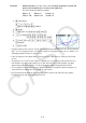
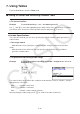
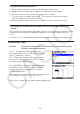
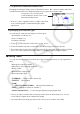
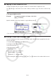
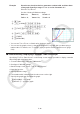
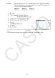

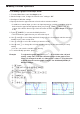
Table Of Contents
- Contents
- Getting Acquainted — Read This First!
- Chapter 1 Basic Operation
- Chapter 2 Manual Calculations
- 1. Basic Calculations
- 2. Special Functions
- 3. Specifying the Angle Unit and Display Format
- 4. Function Calculations
- 5. Numerical Calculations
- 6. Complex Number Calculations
- 7. Binary, Octal, Decimal, and Hexadecimal Calculations with Integers
- 8. Matrix Calculations
- 9. Vector Calculations
- 10. Metric Conversion Calculations
- Chapter 3 List Function
- Chapter 4 Equation Calculations
- Chapter 5 Graphing
- 1. Sample Graphs
- 2. Controlling What Appears on a Graph Screen
- 3. Drawing a Graph
- 4. Saving and Recalling Graph Screen Contents
- 5. Drawing Two Graphs on the Same Screen
- 6. Manual Graphing
- 7. Using Tables
- 8. Modifying a Graph
- 9. Dynamic Graphing
- 10. Graphing a Recursion Formula
- 11. Graphing a Conic Section
- 12. Drawing Dots, Lines, and Text on the Graph Screen (Sketch)
- 13. Function Analysis
- Chapter 6 Statistical Graphs and Calculations
- 1. Before Performing Statistical Calculations
- 2. Calculating and Graphing Single-Variable Statistical Data
- 3. Calculating and Graphing Paired-Variable Statistical Data (Curve Fitting)
- 4. Performing Statistical Calculations
- 5. Tests
- 6. Confidence Interval
- 7. Distribution
- 8. Input and Output Terms of Tests, Confidence Interval, and Distribution
- 9. Statistic Formula
- Chapter 7 Financial Calculation
- Chapter 8 Programming
- Chapter 9 Spreadsheet
- Chapter 10 eActivity
- Chapter 11 Memory Manager
- Chapter 12 System Manager
- Chapter 13 Data Communication
- Chapter 14 Geometry
- Chapter 15 Picture Plot
- Chapter 16 3D Graph Function
- Chapter 17 Python (fx-CG50, fx-CG50 AU only)
- Chapter 18 Distribution (fx-CG50, fx-CG50 AU only)
- Appendix
- Examination Modes
- E-CON4 Application (English)
- 1. E-CON4 Mode Overview
- 2. Sampling Screen
- 3. Auto Sensor Detection (CLAB Only)
- 4. Selecting a Sensor
- 5. Configuring the Sampling Setup
- 6. Performing Auto Sensor Calibration and Zero Adjustment
- 7. Using a Custom Probe
- 8. Using Setup Memory
- 9. Starting a Sampling Operation
- 10. Using Sample Data Memory
- 11. Using the Graph Analysis Tools to Graph Data
- 12. Graph Analysis Tool Graph Screen Operations
- 13. Calling E-CON4 Functions from an eActivity

5-36
Example Store the two functions below, generate a number table, and then draw
a line graph. Specify a range of –3 to 3, and an increment of 1.
Y1 = 3
x
2
– 2, Y2 = x
2
Use the following V-Window settings.
Xmin = 0, Xmax = 6, Xscale = 1
Ymin = –2, Ymax = 10, Yscale = 2
1 m Table
2 !3(V-WIN) awgwbwc
-cwbawcwJ
3 3(TYPE) 1(Y=) dvx-cw
vxw
4 5(SET) -dwdwbwJ
5 6(TABLE)
6 5(GPH-CON)
• You can use Trace, Zoom, or Sketch after drawing a graph.
• You can use the graph screen to change the properties of a graph after you draw using a
number table. For details, see “To change graph properties from the graph screen” (page
5-16).
k Simultaneously Displaying a Number Table and Graph
Specifying “T+G” for “Dual Screen” on the Setup screen makes it possible to display a number
table and graph at the same time.
1. From the Main Menu, enter the Table mode.
2. Configure V-Window settings.
3. On the Setup screen, select “T+G” for “Dual Screen”.
4. Input the function.
5. Specify the table range.
6. The number table is displayed in the sub-screen on the right.
7. Specify the graph type and draw the graph.
5(GPH-CON) ... line graph
6(GPH-PLT) ... plot type graph