
User Manual


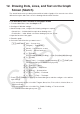
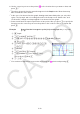


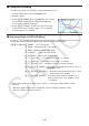
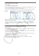

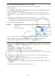
Table Of Contents
- Contents
- Getting Acquainted — Read This First!
- Chapter 1 Basic Operation
- Chapter 2 Manual Calculations
- 1. Basic Calculations
- 2. Special Functions
- 3. Specifying the Angle Unit and Display Format
- 4. Function Calculations
- 5. Numerical Calculations
- 6. Complex Number Calculations
- 7. Binary, Octal, Decimal, and Hexadecimal Calculations with Integers
- 8. Matrix Calculations
- 9. Vector Calculations
- 10. Metric Conversion Calculations
- Chapter 3 List Function
- Chapter 4 Equation Calculations
- Chapter 5 Graphing
- 1. Sample Graphs
- 2. Controlling What Appears on a Graph Screen
- 3. Drawing a Graph
- 4. Saving and Recalling Graph Screen Contents
- 5. Drawing Two Graphs on the Same Screen
- 6. Manual Graphing
- 7. Using Tables
- 8. Modifying a Graph
- 9. Dynamic Graphing
- 10. Graphing a Recursion Formula
- 11. Graphing a Conic Section
- 12. Drawing Dots, Lines, and Text on the Graph Screen (Sketch)
- 13. Function Analysis
- Chapter 6 Statistical Graphs and Calculations
- 1. Before Performing Statistical Calculations
- 2. Calculating and Graphing Single-Variable Statistical Data
- 3. Calculating and Graphing Paired-Variable Statistical Data (Curve Fitting)
- 4. Performing Statistical Calculations
- 5. Tests
- 6. Confidence Interval
- 7. Distribution
- 8. Input and Output Terms of Tests, Confidence Interval, and Distribution
- 9. Statistic Formula
- Chapter 7 Financial Calculation
- Chapter 8 Programming
- Chapter 9 Spreadsheet
- Chapter 10 eActivity
- Chapter 11 Memory Manager
- Chapter 12 System Manager
- Chapter 13 Data Communication
- Chapter 14 Geometry
- Chapter 15 Picture Plot
- Chapter 16 3D Graph Function
- Chapter 17 Python (fx-CG50, fx-CG50 AU only)
- Chapter 18 Distribution (fx-CG50, fx-CG50 AU only)
- Appendix
- Examination Modes
- E-CON4 Application (English)
- 1. E-CON4 Mode Overview
- 2. Sampling Screen
- 3. Auto Sensor Detection (CLAB Only)
- 4. Selecting a Sensor
- 5. Configuring the Sampling Setup
- 6. Performing Auto Sensor Calibration and Zero Adjustment
- 7. Using a Custom Probe
- 8. Using Setup Memory
- 9. Starting a Sampling Operation
- 10. Using Sample Data Memory
- 11. Using the Graph Analysis Tools to Graph Data
- 12. Graph Analysis Tool Graph Screen Operations
- 13. Calling E-CON4 Functions from an eActivity

5-56
k Coordinate Rounding
This function rounds off coordinate values displayed by Trace.
1. From the Main Menu, enter the Graph mode.
2. Draw the graph.
3. Press !2(ZOOM) 6( g) 3(ROUND). This causes
the V-Window settings to be changed automatically
in accordance with the Rnd value.
4. Press !1(TRACE), and then use the cursor keys
to move the pointer along the graph. The coordinates
that now appear are rounded.
k Analyzing Graphs (G-SOLVE Menu)
Pressing !5(G-SOLVE) displays a function menu that contains functions you can use to
analyze the currently displayed graph and obtain the following information.
!5(G-SOLVE)1(ROOT) ... Root of the graph
2(MAX) ... Maximum value of the graph
3(MIN) ... Minimum value of the graph
4(Y-ICEPT) ...
y-intercept of the graph
5(INTSECT) ... Intersection of two graphs
6(g)1(Y-CAL) ...
y-coordinate for a given x-coordinate
6(g)2(X-CAL) ...
x-coordinate for a given y-coordinate
6(g)3(∫d
x)1(∫dx) ... Integration value for a specified range
6(g)3(∫d
x)2(ROOT) ... Integration value between the two or more of
the graph’s roots
6(g)3(∫d
x)3(INTSECT) ... Integration value between the two or more
intersections of two graphs
6(g)3(∫d
x)4(MIXED) ... Integration value between a graph root, a
point of intersection of two graphs, or any
x-coordinate
• Either of the following can cause poor accuracy or even make it impossible to obtain
solutions.
- When the graph of the solution obtained is a point of tangency with the
x-axis
- When a solution is an inflection point