
User Manual
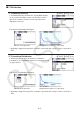
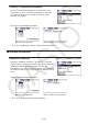
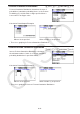
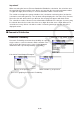
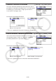

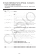
Table Of Contents
- Contents
- Getting Acquainted — Read This First!
- Chapter 1 Basic Operation
- Chapter 2 Manual Calculations
- 1. Basic Calculations
- 2. Special Functions
- 3. Specifying the Angle Unit and Display Format
- 4. Function Calculations
- 5. Numerical Calculations
- 6. Complex Number Calculations
- 7. Binary, Octal, Decimal, and Hexadecimal Calculations with Integers
- 8. Matrix Calculations
- 9. Vector Calculations
- 10. Metric Conversion Calculations
- Chapter 3 List Function
- Chapter 4 Equation Calculations
- Chapter 5 Graphing
- 1. Sample Graphs
- 2. Controlling What Appears on a Graph Screen
- 3. Drawing a Graph
- 4. Saving and Recalling Graph Screen Contents
- 5. Drawing Two Graphs on the Same Screen
- 6. Manual Graphing
- 7. Using Tables
- 8. Modifying a Graph
- 9. Dynamic Graphing
- 10. Graphing a Recursion Formula
- 11. Graphing a Conic Section
- 12. Drawing Dots, Lines, and Text on the Graph Screen (Sketch)
- 13. Function Analysis
- Chapter 6 Statistical Graphs and Calculations
- 1. Before Performing Statistical Calculations
- 2. Calculating and Graphing Single-Variable Statistical Data
- 3. Calculating and Graphing Paired-Variable Statistical Data (Curve Fitting)
- 4. Performing Statistical Calculations
- 5. Tests
- 6. Confidence Interval
- 7. Distribution
- 8. Input and Output Terms of Tests, Confidence Interval, and Distribution
- 9. Statistic Formula
- Chapter 7 Financial Calculation
- Chapter 8 Programming
- Chapter 9 Spreadsheet
- Chapter 10 eActivity
- Chapter 11 Memory Manager
- Chapter 12 System Manager
- Chapter 13 Data Communication
- Chapter 14 Geometry
- Chapter 15 Picture Plot
- Chapter 16 3D Graph Function
- Chapter 17 Python (fx-CG50, fx-CG50 AU only)
- Chapter 18 Distribution (fx-CG50, fx-CG50 AU only)
- Appendix
- Examination Modes
- E-CON4 Application (English)
- 1. E-CON4 Mode Overview
- 2. Sampling Screen
- 3. Auto Sensor Detection (CLAB Only)
- 4. Selecting a Sensor
- 5. Configuring the Sampling Setup
- 6. Performing Auto Sensor Calibration and Zero Adjustment
- 7. Using a Custom Probe
- 8. Using Setup Memory
- 9. Starting a Sampling Operation
- 10. Using Sample Data Memory
- 11. Using the Graph Analysis Tools to Graph Data
- 12. Graph Analysis Tool Graph Screen Operations
- 13. Calling E-CON4 Functions from an eActivity

6-65
Calculation Result Output Examples
When a list is specified When variable (
x ) is specified
• There is no graphing for Hypergeometric Cumulative Distribution.
• Inverse Hypergeometric Cumulative Distribution
5(DIST) 6( g) 3(HYPRGEO) 3(InvH)
Inverse Hypergeometric Cumulative Distribution calculates
the minimum number of trials of a hypergeometric
cumulative probability distribution for specified values.
Calculation Result Output Examples
When a list is specified When variable (
x ) is specified
• There is no graphing for Inverse Hypergeometric Cumulative Distribution.
Important!
When executing the Inverse Hypergeometric Cumulative Distribution calculation, the calculator
uses the specified Area value and the value that is one less than the Area value minimum
number of significant digits ( `Area value) to calculate minimum number of trials values.
The results are assigned to system variables
x Inv (calculation result using Area) and `x Inv
(calculation result using `Area). The calculator always displays the
x Inv value only. However,
when the x Inv and `x Inv values are different, the message will appear with both values.
The calculation results of Inverse Hypergeometric Cumulative Distribution are integers.
Accuracy may be reduced when the Area value has 10 or more digits. Note that even a slight
difference in calculation accuracy affects calculation results. If a warning message appears,
check the displayed values.