User Manual

ManualsBrandsCASIO ManualsCalculatorsFX-CG50

271

272

273

274

275

276

277

278

279

280

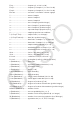
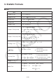
Table Of Contents

Contents
Getting Acquainted — Read This First!
Chapter 1 Basic Operation
- 1. Keys
- 2. Display
- 3. Inputting and Editing Calculations
- 4. Using the Math Input/Output Mode
- 5. Option (OPTN) Menu
- 6. Variable Data (VARS) Menu
- 7. Program (PRGM) Menu
- 8. Using the Setup Screen
- 9. Using Screen Capture
- 10. When you keep having problems...
Chapter 2 Manual Calculations
- 1. Basic Calculations
- 2. Special Functions
- 3. Specifying the Angle Unit and Display Format
- 4. Function Calculations
- 5. Numerical Calculations
- 6. Complex Number Calculations
- 7. Binary, Octal, Decimal, and Hexadecimal Calculations with Integers
- 8. Matrix Calculations
- 9. Vector Calculations
- 10. Metric Conversion Calculations
Chapter 3 List Function
- 1. Inputting and Editing a List
- 2. Manipulating List Data
- 3. Arithmetic Calculations Using Lists
- 4. Switching between List Files
- 5. Using CSV Files
Chapter 4 Equation Calculations
- 1. Simultaneous Linear Equations
- 2. High-order Equations from 2nd to 6th Degree
- 3. Solve Calculations
Chapter 5 Graphing
- 1. Sample Graphs
- 2. Controlling What Appears on a Graph Screen
- 3. Drawing a Graph
- 4. Saving and Recalling Graph Screen Contents
- 5. Drawing Two Graphs on the Same Screen
- 6. Manual Graphing
- 7. Using Tables
- 8. Modifying a Graph
- 9. Dynamic Graphing
- 10. Graphing a Recursion Formula
- 11. Graphing a Conic Section
- 12. Drawing Dots, Lines, and Text on the Graph Screen (Sketch)
- 13. Function Analysis
Chapter 6 Statistical Graphs and Calculations
- 1. Before Performing Statistical Calculations
- 2. Calculating and Graphing Single-Variable Statistical Data
- 3. Calculating and Graphing Paired-Variable Statistical Data (Curve Fitting)
- 4. Performing Statistical Calculations
- 5. Tests
- 6. Confidence Interval
- 7. Distribution
- 8. Input and Output Terms of Tests, Confidence Interval, and Distribution
- 9. Statistic Formula
Chapter 7 Financial Calculation
- 1. Before Performing Financial Calculations
- 2. Simple Interest
- 3. Compound Interest
- 4. Cash Flow (Investment Appraisal)
- 5. Amortization
- 6. Interest Rate Conversion
- 7. Cost, Selling Price, Margin
- 8. Day/Date Calculations
- 9. Depreciation
- 10. Bond Calculations
- 11. Financial Calculations Using Functions
Chapter 8 Programming
- 1. Basic Programming Steps
- 2. Program Mode Function Keys
- 3. Editing Program Contents
- 4. File Management
- 5. Command Reference
- 6. Using Calculator Functions in Programs
- 7. Program Mode Command List
- 8. CASIO Scientific Function Calculator Special Commands <=> Text Conversion Table
- 9. Program Library
Chapter 9 Spreadsheet
- 1. Spreadsheet Basics and the Function Menu
- 2. Basic Spreadsheet Operations
- 3. Using Special Spreadsheet Mode Commands
- 4. Conditional Formatting
- 5. Drawing Statistical Graphs, and Performing Statistical and Regression Calculations
- 6. Spreadsheet Mode Memory
Chapter 10 eActivity
- 1. eActivity Overview
- 2. eActivity Function Menus
- 3. eActivity File Operations
- 4. Inputting and Editing Data
Chapter 11 Memory Manager
- 1. Using the Memory Manager
Chapter 12 System Manager
- 1. Using the System Manager
- 2. System Settings
Chapter 13 Data Communication
- 1. Performing Data Communication between the Calculator and a Personal Computer
- 2. Performing Data Communication between Two Calculators
- 3. Connecting the Calculator to a Projector
Chapter 14 Geometry
- 1. Geometry Mode Overview
- 2. Drawing and Editing Objects
- 3. Controlling the Appearance of the Geometry Window
- 4. Using Text and Labels in a Screen Image
- 5. Using the Measurement Box
- 6. Working with Animations
Chapter 15 Picture Plot
- 1. Picture Plot Function Menus
- 2. Managing Picture Plot Files
- 3. Using the Plot Function
- 4. Using the Plot List
- 5. Common Functions with the Graph Mode
Chapter 16 3D Graph Function
- 1. Example of Drawing in the 3D Graph Mode
- 2. 3D View Window
- 3. 3D Graph Function Lis
- 4. 3D Graph Function Selection Screen
- 5. 3D Graph Screen
Chapter 17 Python (fx-CG50, fx-CG50 AU only)
- 1. Python Mode Overview
- 2. Python Function Menu
- 3. Inputting Text and Commands
- 4. Using the SHELL
- 5. Using Draw Functions (casioplot Module)
- 6. Editing a py File
- 7. File Management (Searching For and Deleting Files)
- 8. File Compatibility
- 9. Sample Scripts
Chapter 18 Distribution (fx-CG50, fx-CG50 AU only)
- 1. Distribution Mode Overview
- 2. Distribution Function Menu
- 3. Other Operations
- 4. Distribution Examples
Appendix
- 1. Error Message Table
- 2. Input Ranges
Examination Modes
E-CON4 Application (English)
- 1. E-CON4 Mode Overview
- 2. Sampling Screen
- 3. Auto Sensor Detection (CLAB Only)
- 4. Selecting a Sensor
- 5. Configuring the Sampling Setup
- 6. Performing Auto Sensor Calibration and Zero Adjustment
- 7. Using a Custom Probe
- 8. Using Setup Memory
- 9. Starting a Sampling Operation
- 10. Using Sample Data Memory
- 11. Using the Graph Analysis Tools to Graph Data
- 12. Graph Analysis Tool Graph Screen Operations
- 13. Calling E-CON4 Functions from an eActivity

6-72

k Distribution (Discrete)

Distribution Probability

Binomial Distribution

p(x) =

nCxp

(1–p)

n – x

(x = 0, 1, ·······, n)

n : number of trials

Poisson Distribution

(x = 0, 1, 2, ···)

p(x) =

–

: mean (

> 0)

Geometric Distribution

p(x)

= p(1– p)

x – 1

(x = 1, 2, 3, ···)

Hypergeometric

Distribution

p(x) =

MCx × N – MCn – x

n : Number of trials from population (0  n integer)

M : Number of successes in population (0  M integer)

N : Population size ( n  N , M  N integer)

Distribution

Cumulative Distribution

Inverse Cumulative Distribution

Binomial Distribution

p =

p(x)

x=Lower

Upper

p H

p(x)

x=0

Poisson Distribution

Geometric Distribution

p =

p(x)

x=Lower

Upper

p H

p(x)

x=1

Hypergeometric

Distribution

p =

p(x)

x=Lower

Upper

p H

p(x)

x=0