
User Manual
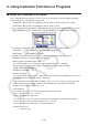

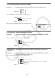
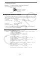
Table Of Contents
- Contents
- Getting Acquainted — Read This First!
- Chapter 1 Basic Operation
- Chapter 2 Manual Calculations
- 1. Basic Calculations
- 2. Special Functions
- 3. Specifying the Angle Unit and Display Format
- 4. Function Calculations
- 5. Numerical Calculations
- 6. Complex Number Calculations
- 7. Binary, Octal, Decimal, and Hexadecimal Calculations with Integers
- 8. Matrix Calculations
- 9. Vector Calculations
- 10. Metric Conversion Calculations
- Chapter 3 List Function
- Chapter 4 Equation Calculations
- Chapter 5 Graphing
- 1. Sample Graphs
- 2. Controlling What Appears on a Graph Screen
- 3. Drawing a Graph
- 4. Saving and Recalling Graph Screen Contents
- 5. Drawing Two Graphs on the Same Screen
- 6. Manual Graphing
- 7. Using Tables
- 8. Modifying a Graph
- 9. Dynamic Graphing
- 10. Graphing a Recursion Formula
- 11. Graphing a Conic Section
- 12. Drawing Dots, Lines, and Text on the Graph Screen (Sketch)
- 13. Function Analysis
- Chapter 6 Statistical Graphs and Calculations
- 1. Before Performing Statistical Calculations
- 2. Calculating and Graphing Single-Variable Statistical Data
- 3. Calculating and Graphing Paired-Variable Statistical Data (Curve Fitting)
- 4. Performing Statistical Calculations
- 5. Tests
- 6. Confidence Interval
- 7. Distribution
- 8. Input and Output Terms of Tests, Confidence Interval, and Distribution
- 9. Statistic Formula
- Chapter 7 Financial Calculation
- Chapter 8 Programming
- Chapter 9 Spreadsheet
- Chapter 10 eActivity
- Chapter 11 Memory Manager
- Chapter 12 System Manager
- Chapter 13 Data Communication
- Chapter 14 Geometry
- Chapter 15 Picture Plot
- Chapter 16 3D Graph Function
- Chapter 17 Python (fx-CG50, fx-CG50 AU only)
- Chapter 18 Distribution (fx-CG50, fx-CG50 AU only)
- Appendix
- Examination Modes
- E-CON4 Application (English)
- 1. E-CON4 Mode Overview
- 2. Sampling Screen
- 3. Auto Sensor Detection (CLAB Only)
- 4. Selecting a Sensor
- 5. Configuring the Sampling Setup
- 6. Performing Auto Sensor Calibration and Zero Adjustment
- 7. Using a Custom Probe
- 8. Using Setup Memory
- 9. Starting a Sampling Operation
- 10. Using Sample Data Memory
- 11. Using the Graph Analysis Tools to Graph Data
- 12. Graph Analysis Tool Graph Screen Operations
- 13. Calling E-CON4 Functions from an eActivity

8-28
6. Using Calculator Functions in Programs
k Using Color Commands in a Program
Color commands let you specify colors for on-screen lines, text, and other display elements.
The following color commands are supported.
RUN Mode: Black, Blue, Red, Magenta, Green, Cyan, Yellow, ColorAuto, ColorClr
BASE Mode: Black, Blue, Red, Magenta, Green, Cyan, Yellow
• Color commands are input with the dialog box shown below, which appears when you press
!f(FORMAT)b(Color Command) (!f(FORMAT) in a BASE Mode program).
For example, the following key operation would input the color command Blue.
RUN Mode: !f(FORMAT)b(Color Command)c(Blue)
BASE Mode: !f(FORMAT)c(Blue)
• Except for ColorAuto and ColorClr, color commands can be used in a program in
combination with the commands described below.
- Manual graph commands (page 5-25)
You can specify the color of a manual graph by placing a color command
before “Graph Y=” or any other graph commands that can be input following
!4(SKETCH)5(GRAPH).
Example: Red Graph Y = X
2
− 1
- Sketch Commands
You can specify the draw color of a figure drawn with a Sketch command by placing a color
command before the following Sketch commands.
Tangent, Normal, Inverse, PlotOn, PlotChg, F-Line, Line, Circle, Vertical, Horizontal, Text,
PxlOn, PxlChg, SketchNormal, SketchThick, SketchBroken, SketchDot, SketchThin
Example: Green SketchThin Circle 2, 1, 2
- List Command
You can specify a color for a list using the syntaxes shown below.
<color command> List
n (n = 1 to 26)
<color command> List "sub name"
You can specify a color for a specific element in a list using the syntaxes shown below.
<color command> List
n [<element number>] (n = 1 to 26)
<color command> List "sub name" [<element number>]
Example: Blue List 1
Red List 1 [3]