
User Manual
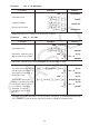
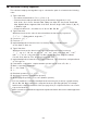
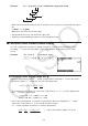
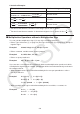
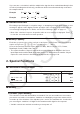
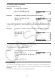
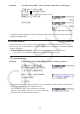
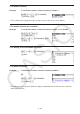
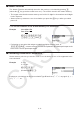
Table Of Contents
- Contents
- Getting Acquainted — Read This First!
- Chapter 1 Basic Operation
- Chapter 2 Manual Calculations
- 1. Basic Calculations
- 2. Special Functions
- 3. Specifying the Angle Unit and Display Format
- 4. Function Calculations
- 5. Numerical Calculations
- 6. Complex Number Calculations
- 7. Binary, Octal, Decimal, and Hexadecimal Calculations with Integers
- 8. Matrix Calculations
- 9. Vector Calculations
- 10. Metric Conversion Calculations
- Chapter 3 List Function
- Chapter 4 Equation Calculations
- Chapter 5 Graphing
- 1. Sample Graphs
- 2. Controlling What Appears on a Graph Screen
- 3. Drawing a Graph
- 4. Saving and Recalling Graph Screen Contents
- 5. Drawing Two Graphs on the Same Screen
- 6. Manual Graphing
- 7. Using Tables
- 8. Modifying a Graph
- 9. Dynamic Graphing
- 10. Graphing a Recursion Formula
- 11. Graphing a Conic Section
- 12. Drawing Dots, Lines, and Text on the Graph Screen (Sketch)
- 13. Function Analysis
- Chapter 6 Statistical Graphs and Calculations
- 1. Before Performing Statistical Calculations
- 2. Calculating and Graphing Single-Variable Statistical Data
- 3. Calculating and Graphing Paired-Variable Statistical Data (Curve Fitting)
- 4. Performing Statistical Calculations
- 5. Tests
- 6. Confidence Interval
- 7. Distribution
- 8. Input and Output Terms of Tests, Confidence Interval, and Distribution
- 9. Statistic Formula
- Chapter 7 Financial Calculation
- Chapter 8 Programming
- Chapter 9 Spreadsheet
- Chapter 10 eActivity
- Chapter 11 Memory Manager
- Chapter 12 System Manager
- Chapter 13 Data Communication
- Chapter 14 Geometry
- Chapter 15 Picture Plot
- Chapter 16 3D Graph Function
- Chapter 17 Python (fx-CG50, fx-CG50 AU only)
- Chapter 18 Distribution (fx-CG50, fx-CG50 AU only)
- Appendix
- Examination Modes
- E-CON4 Application (English)
- 1. E-CON4 Mode Overview
- 2. Sampling Screen
- 3. Auto Sensor Detection (CLAB Only)
- 4. Selecting a Sensor
- 5. Configuring the Sampling Setup
- 6. Performing Auto Sensor Calibration and Zero Adjustment
- 7. Using a Custom Probe
- 8. Using Setup Memory
- 9. Starting a Sampling Operation
- 10. Using Sample Data Memory
- 11. Using the Graph Analysis Tools to Graph Data
- 12. Graph Analysis Tool Graph Screen Operations
- 13. Calling E-CON4 Functions from an eActivity

2-2
Example 1 100 ÷ 6 = 16.66666666...
Condition Operation Display
100 /6 w
16.66666667
4 decimal places
!m(SET UP) ff
1(Fix) ewJw
16.6667
5 significant digits
!m(SET UP) ff
2(Sci) fwJw
1.6667 × 10
01
Cancels specification
!m(SET UP) ff
3(Norm) Jw
16.66666667
*
1
Displayed values are rounded off to the place you specify.
Example 2 200 ÷ 7 × 14 = 400
Condition Operation Display
200 /7 *14 w
400
3 decimal places
!m(SET UP) ff
1(Fix) dwJw
400.000
Calculation continues using
display capacity of 10 digits
200 /7 w
*
14 w
28.571
Ans ×
I
400.000
• If the same calculation is performed using the specified number of digits:
200 /7 w
28.571
The value stored internally is
rounded off to the number of
decimal places specified on
the Setup screen.
K6( g) 4(NUMERIC) 4(Rnd) w
*
14 w
28.571
Ans ×
I
399.994
200 /7 w
28.571
You can also specify the
number of decimal places for
rounding of internal values
for a specific calculation.
(Example: To specify
rounding to two decimal
places)
6( g) 1(RndFix) !-(Ans) ,2 )
w
*
14 w
RndFix(Ans,2)
28.570
Ans ×
I
399.980
• You cannot use a first derivative, second derivative, integration, Σ , maximum/minimum value,
Solve, RndFix or log
a
b calculation expression inside of a RndFix calculation term.
*
1
*
1