
User Manual
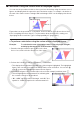
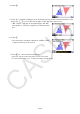
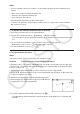
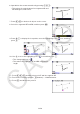
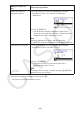

Table Of Contents
- Contents
- Getting Acquainted — Read This First!
- Chapter 1 Basic Operation
- Chapter 2 Manual Calculations
- 1. Basic Calculations
- 2. Special Functions
- 3. Specifying the Angle Unit and Display Format
- 4. Function Calculations
- 5. Numerical Calculations
- 6. Complex Number Calculations
- 7. Binary, Octal, Decimal, and Hexadecimal Calculations with Integers
- 8. Matrix Calculations
- 9. Vector Calculations
- 10. Metric Conversion Calculations
- Chapter 3 List Function
- Chapter 4 Equation Calculations
- Chapter 5 Graphing
- 1. Sample Graphs
- 2. Controlling What Appears on a Graph Screen
- 3. Drawing a Graph
- 4. Saving and Recalling Graph Screen Contents
- 5. Drawing Two Graphs on the Same Screen
- 6. Manual Graphing
- 7. Using Tables
- 8. Modifying a Graph
- 9. Dynamic Graphing
- 10. Graphing a Recursion Formula
- 11. Graphing a Conic Section
- 12. Drawing Dots, Lines, and Text on the Graph Screen (Sketch)
- 13. Function Analysis
- Chapter 6 Statistical Graphs and Calculations
- 1. Before Performing Statistical Calculations
- 2. Calculating and Graphing Single-Variable Statistical Data
- 3. Calculating and Graphing Paired-Variable Statistical Data (Curve Fitting)
- 4. Performing Statistical Calculations
- 5. Tests
- 6. Confidence Interval
- 7. Distribution
- 8. Input and Output Terms of Tests, Confidence Interval, and Distribution
- 9. Statistic Formula
- Chapter 7 Financial Calculation
- Chapter 8 Programming
- Chapter 9 Spreadsheet
- Chapter 10 eActivity
- Chapter 11 Memory Manager
- Chapter 12 System Manager
- Chapter 13 Data Communication
- Chapter 14 Geometry
- Chapter 15 Picture Plot
- Chapter 16 3D Graph Function
- Chapter 17 Python (fx-CG50, fx-CG50 AU only)
- Chapter 18 Distribution (fx-CG50, fx-CG50 AU only)
- Appendix
- Examination Modes
- E-CON4 Application (English)
- 1. E-CON4 Mode Overview
- 2. Sampling Screen
- 3. Auto Sensor Detection (CLAB Only)
- 4. Selecting a Sensor
- 5. Configuring the Sampling Setup
- 6. Performing Auto Sensor Calibration and Zero Adjustment
- 7. Using a Custom Probe
- 8. Using Setup Memory
- 9. Starting a Sampling Operation
- 10. Using Sample Data Memory
- 11. Using the Graph Analysis Tools to Graph Data
- 12. Graph Analysis Tool Graph Screen Operations
- 13. Calling E-CON4 Functions from an eActivity

14-57
Note
• You can repeat the above procedure to create multiple points that move simultaneously.
Try this:
- Draw a line segment and plot another point.
- Select the line segment and the point.
- Repeat steps 2 and 3 above.
Notice that both animations go at the same time!
• To start a new animation, perform the procedure under “To replace the current animation
with a new one” below.
u To replace the current animation with a new one
1. Select the point and curve for the new animation.
2. Perform the following operation: 6(Animate) – 2:Replace Anima.
• This discards the current animations and sets up an animation for a new point and curve
set.
3. To execute the new animation, perform either of the following operations:
6(Animate) – 5:Go (once) or 6(Animate) – 6:Go (repeat)
4. To stop the animation, press J or o.
u To trace a locus of points
Note
Using trace leaves a trail of points when the animation is run.
Example: To use the Trace command to draw a parabola
A parabola is the locus of points equidistant from a point (the focus) and a line (the directrix).
Use the Trace command to draw a parabola using a line segment (AB) as the directrix and a
point (C) as the focus.
1. Draw a line segment AB and plot point C, which is not on line segment AB.
2. Plot point D, which should also not be on line segment AB, but should be on the same side
of the line segment as point C.
3. Draw a line segment that connects point D with point C.
4. Draw another line segment that connects point D with line
segment AB. This is line segment DE.
5. Select line segments AB and DE, and then press J.
• This displays the measurement box, which shows the angle between line segments AB
and DE.