
User Manual
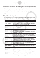
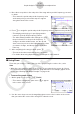
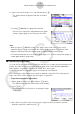
Table Of Contents
- Sommaire
- Familiarisation — À lire en premier !
- Chapitre 1 Opérations de base
- 1. Touches
- 2. Affichage
- 3. Saisie et édition de calculs
- 4. Utilisation du mode d’écriture mathématique
- 5. Menu d’options (OPTN)
- 6. Menu de données de variables (VARS)
- 7. Menu de programmation (PRGM)
- 8. Utilisation de l’écran de configuration
- 9. Utilisation de la capture d’écran
- 10. En cas de problème persistant...
- Chapitre 2 Calculs manuels
- 1. Calculs de base
- 2. Fonctions spéciales
- 3. Spécification de l’unité d’angle et du format d’affichage
- 4. Calculs de fonctions
- 5. Calculs numériques
- 6. Calculs avec nombres complexes
- 7. Calculs binaire, octal, décimal et hexadécimal avec entiers
- 8. Calculs matriciels
- 9. Calculs vectoriels
- 10. Calculs de conversion métrique
- Chapitre 3 Listes
- Chapitre 4 Calcul d’équations
- Chapitre 5 Représentation graphique de fonctions
- 1. Exemples de graphes
- 2. Contrôle des paramètres apparaissant sur l’écran d’un graphe
- 3. Tracé d’un graphe
- 4. Enregistrement et rappel du contenu de l’écran du graphe
- 5. Tracé de deux graphes sur le même écran
- 6. Représentation graphique manuelle
- 7. Utilisation des tableaux
- 8. Modification d’un graphe
- 9. Représentation graphique dynamique
- 10. Représentation graphique d’une formule de récurrence
- 11. Tracé du graphe d’une section conique
- 12. Tracé de points, de lignes et de texte sur l’écran du graphe (Sketch)
- 13. Analyse de fonctions
- Chapitre 6 Graphes et calculs statistiques
- 1. Avant d’effectuer des calculs statistiques
- 2. Calcul et représentation graphique de données statistiques à variable unique
- 3. Calcul et représentation graphique de données statistiques à variable double (Ajustement de courbe)
- 4. Exécution de calculs statistiques
- 5. Tests
- 6. Intervalle de confiance
- 7. Distribution
- 8. Termes des tests d’entrée et sortie, intervalle de confiance et distribution
- 9. Formule statistique
- Chapitre 7 Calculs financiers
- 1. Avant d’effectuer des calculs financiers
- 2. Intérêt simple
- 3. Intérêt composé
- 4. Flux de trésorerie (Évaluation d’investissement)
- 5. Amortissement
- 6. Conversion de taux d’intérêt
- 7. Coût, prix de vente, marge
- 8. Calculs de jours/date
- 9. Dépréciation
- 10. Calculs d’obligations
- 11. Calculs financiers en utilisant des fonctions
- Chapitre 8 Programmation
- 1. Étapes élémentaires de la programmation
- 2. Touches de fonction du mode Programme
- 3. Édition du contenu d’un programme
- 4. Gestion de fichiers
- 5. Guide des commandes
- 6. Utilisation des fonctions de la calculatrice dans un programme
- 7. Liste des commandes du mode Programme
- 8. Tableau de conversion des commandes spéciales de la calculatrice scientifique CASIO <=> Texte
- 9. Bibliothèque de programmes
- Chapitre 9 Feuille de Calcul
- Chapitre 10 L’eActivity
- Chapitre 11 Gestionnaire de mémoire
- Chapitre 12 Menu de réglages du système
- Chapitre 13 Communication de données
- Chapitre 14 Géométrie
- Chapitre 15 Plot Image (Tracé sur image)
- Chapitre 16 Fonction du graphe 3D
- Chapitre 17 Python
- 1. Aperçu du mode Python
- 2. Menu de fonctions de Python
- 3. Saisie de texte et de commandes
- 4. Utilisation du SHELL
- 5. Utilisation des fonctions de tracé (module casioplot)
- 6. Modification d’un fichier py
- 7. Gestion de dossiers (recherche et suppression de fichiers)
- 8. Compatibilité de fichier
- 9. Exemples de scripts
- Chapitre 18 Distribution
- Appendice
- Mode Examen
- E-CON4 Application (English)
- 1. E-CON4 Mode Overview
- 2. Sampling Screen
- 3. Auto Sensor Detection (CLAB Only)
- 4. Selecting a Sensor
- 5. Configuring the Sampling Setup
- 6. Performing Auto Sensor Calibration and Zero Adjustment
- 7. Using a Custom Probe
- 8. Using Setup Memory
- 9. Starting a Sampling Operation
- 10. Using Sample Data Memory
- 11. Using the Graph Analysis Tools to Graph Data
- 12. Graph Analysis Tool Graph Screen Operations
- 13. Calling E-CON4 Functions from an eActivity

ε-40
Graph Analysis Tool Graph Screen Operations
Key Operation Description
K5(Y=fx)
Displays the graph relation list, which lets you select a Y=f(x)
graph to overlay on the sampled result graph. See “Overlaying a
Y=f(x) Graph on a Sampled Result Graph” on page
ε-46.
K6(SPEAKER)
Starts an operation for outputting a specific range of a sound data
waveform graph from the speaker (EA-200 only). See “Outputting
a Specific Range of a Graph from the Speaker” on page
ε-48.
k Scrolling the Graph Screen
Press the cursor keys while the graph screen is on the display scrolls the graph left, right, up,
or down.
Note
• The cursor keys perform different operations besides scrolling while a trace or graph
operation is in progress. To perform a graph screen scroll operation in this case, press J
to cancel the trace or graph operation, and then press the cursor keys.
k Using Trace
Trace displays a crosshair pointer on the displayed graph along with the coordinates of the
current cursor position. You can use the cursor keys to move the pointer along the graph.
You can also use trace to obtain the periodic frequency value for a particular range, and
assign the range (time) and periodic frequency values in separate Alpha memory variables.
• To use trace
1. On the graph screen, press !1(TRACE).
• This causes a trace pointer to appear on the graph.
The coordinates of the current trace pointer location
are also shown on the display.
2. Use the d and e cursor keys to move the trace pointer along the graph to the location
you want.
• The coordinate values change in accordance with the trace pointer movement.
• You can exit the trace pointer at any time by pressing J.
• To obtain the periodic frequency value
1. Use the procedure under “To use trace” above to start a trace operation.
2. Move the trace pointer to the start point of the range whose periodic frequency you want
to obtain, and then press w.