User guide

I
2
T Time Limit Algorithm CME 2 User Guide
194 Copley Controls
I
2
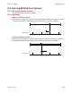
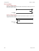
T Example: Plot Diagrams
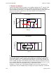
The plots that follow show the response of an amplifier (configured w/ I
2
T setpoint = 108
A
2
S) to a given current command. For this example, DC output currents are shown in
order to simplify the waveforms. The algorithm essentially calculates the RMS value of the
output current, and thus operates the same way regardless of the output current
frequency and wave shape.
A)
I
2
T current limit
0
2
4
6
8
10
12
14
16
0 1 2 3 4 5 6 7
Time (S)
Current (A)
I_commanded
I_actual
B)
I
2
T Accumulator
0
20
40
60
80
100
120
0 1 2 3 4 5 6 7
Time (S)
I
2
T energy (A
2
-S)
I^2T Setpoint
I^2T Accumulator
At time 0, plot diagram A shows that the actual output current follows the commanded
current. Note that the current is higher than the continuous current limit setting of 6 A.
Under this condition, the I
2
T Accumulator Variable begins increasing from its initial value
of zero. Initially, the output current linearly increases from 6 A up to 12 A over the course
of 1.2 seconds. During this same period, the I
2
T Accumulator Variable increases in a non-
linear fashion because of its dependence on the square of the current.
At about 1.6 seconds, the I
2
T Accumulator Variable reaches a values equal to the I
2
T
setpoint. At this time, the amplifier limits the output current to the continuous current limit