Dell HPC System for Manufacturing—System Architecture and Application Performance This Dell technical white paper describes the architecture of the Dell HPC System for Manufacturing and discusses performance benchmarking results and analysis for ANSYS Fluent, ANSYS Mechanical, CD-adapco, a Siemens Business, STARCCM+, LSTC LS-DYNA, NICE DCV, and EnginFrame.
Revisions Date Description July 2016 Initial release THIS WHITE PAPER IS FOR INFORMATIONAL PURPOSES ONLY, AND MAY CONTAIN TYPOGRAPHICAL ERRORS AND TECHNICAL INACCURACIES. THE CONTENT IS PROVIDED AS IS, WITHOUT EXPRESS OR IMPLIED WARRANTIES OF ANY KIND. Copyright © 2016 Dell Inc. All rights reserved. Dell and the Dell logo are trademarks of Dell Inc. in the United States and/or other jurisdictions. All other marks and names mentioned herein may be trademarks of their respective companies.
Contents 1 Introduction .....................................................................................................................................................................................5 2 System Building Blocks ................................................................................................................................................................ 6 2.1 Infrastructure Servers ......................................................................................
Executive Summary This technical white paper describes the architecture of the Dell HPC System for Manufacturing, which consists of building blocks configured specifically for applications in the manufacturing domain. Detailed performance results with sample CFD and FEA applications, and power characteristics of the system are presented in this document. Virtual Desktop Infrastructure (VDI) capability is also described and validated.
1 Introduction This technical white paper describes the Dell HPC System for Manufacturing. The Dell HPC System for Manufacturing is designed and configured specifically for customers in the manufacturing domain. This system uses a flexible building block approach, where individual building blocks can be combined to build HPC systems which are ideal for customer specific work-loads and use cases.
2 System Building Blocks The Dell HPC System for Manufacturing is assembled by using preconfigured building blocks. The available building blocks are infrastructure servers, storage, networking, Virtual Desktop Infrastructure (VDI), and application specific compute building blocks. These building blocks are preconfigured to provide good performance for typical applications and workloads within the manufacturing domain.
2.2 Explicit Building Blocks Explicit Building Block (EBB) servers are typically used for Computational Fluid Dynamics (CFD) and explicit Finite Element Analysis (FEA) solvers such as Abaqus/Explicit, Altair® RADIOSS™, ANSYS Fluent, CD-adapco STAR-CCM+, ESI PAM-CRASH, Exa PowerFLOW®, LSTC LS-DYNA, and OpenFOAM®. These software applications typically scale well across many processor cores and multiple servers.
2.3 Implicit Building Blocks Implicit Building Block (IBB) servers are typically used for implicit FEA solvers such as Abaqus/Standard, Altair OptiStruct®, ANSYS Mechanical™, MSC™ Nastran™, and NX® Nastran. These applications typically have large memory requirements and do not scale to as many cores as the EBB applications. They also often have a large drive I/O component.
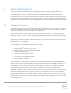
The recommended configuration for IGPGPUBBs is: • • • • • • • • • Dell PowerEdge R730 server Dual Intel Xeon E5-2680 v4 processors 256 GB of memory, 16 x 16 GB 2400 MT/s DIMMs PERC H730 RAID controller 8 x 300 GB 15K SAS drives in RAID 0 Dell iDRAC8 Express 2 x 1100 W PSUs One NVIDIA® Tesla® K80 EDR InfiniBand (optional) The recommended configuration for the IGPGPUBB servers is described here. A Dell PowerEdge R730 server is required to support the NVIDIA Tesla K80.
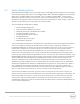
• • • • • • 4 x 600 GB 10K SAS drives in RAID 0 (for local temporary storage) QLogic 10 GbE Network Daughter Card (NDC) Dell iDRAC8 Express 2 x 1100 W PSUs One NVIDIA GRID® K2 EDR InfiniBand (optional) The recommended configuration for the VDI server is described here. A PowerEdge R730 is required to support the NVIDIA GRID K2 which is used to provide hardware accelerated 3D graphics. The Intel Xeon E5-2680 v4 with 14 cores at 2.4 GHz (maximum all-core turbo of 2.
2.7 Dell IEEL Storage Dell IEEL storage is an Intel Enterprise Edition for Lustre (IEEL) based storage solution consisting of a management station, Lustre metadata servers, Lustre object storage servers, and the associated backend storage. The management station provides end-to-end management and monitoring for the entire Lustre storage system. The Dell IEEL storage solution provides a parallel file system with options of 480 TB or 960 TB raw storage disk space.
SB7790 36-port EDR InfiniBand switches. The number of switches required depends on the size of the cluster and the blocking ratio of the fabric. 2.9 VDI Software The VDI software is installed on the VDI servers and provides GPU accelerated remote visualization capabilities. NICE DCV with NICE EnginFrame is the recommended VDI software stack for the Dell HPC System for Manufacturing. 2.10 Cluster Software The Cluster Software is used to install and monitor the system’s compute servers.
3 Reference System The reference system was assembled in the Dell HPC Innovation Lab by using the system building blocks described in Section 2. The building blocks used for the reference system are listed in Table 1.
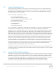
The software versions used for the reference system are listed in Table 3. Software Versions Component Version Operating System RHEL 7.2 Kernel 3.10.0-327.el7.x86_64 OFED Mellanox 3.2-2.0.0.0 Bright Cluster Manager 7.2 with RHEL 7.2 (Dell version) ANSYS Fluent v17.1 ANSYS Fluent Benchmarks v15 and v16 ANSYS Mechanical v17.1 ANSYS Mechanical Benchmarks v17.0 CD-adapco STAR-CCM+ 11.02.010 mixed precision CD-adapco STAR-CCM+ Benchmarks HPL Benchmark cases as listed NVIDIA Driver v1.5.2.
4 System Performance This section presents the performance results obtained from the reference system described in Section 3. Basic performance of the servers was measured first, prior to any application benchmarking. This was done to ensure that individual server sub-systems were performing as expected and that the systems were stable.
building blocks is 11%; however, the slowest result is still within specification for the relevant processor model. Results of running HPL in parallel on the eight Explicit building blocks are presented in Figure 2. This bar chart shows HPL performance from one to eight servers. This test demonstrates good scalability of the system with up to eight Explicit building blocks.
4.3 ANSYS Fluent ANSYS Fluent is a multi-physics Computational Fluid Dynamics (CFD) software commonly used in multiple engineering disciplines. CFD applications typically scale well across multiple processor cores and servers, have modest memory capacity requirements, and perform minimal disk I/O while solving. For these types of application characteristics, the Explicit building block servers are appropriate.
and some models run much faster than others depending on the number of cells in the model, type of solver used and physics of the problem. Combustor_71m, f1_racecar_140m and open_racecar280m are large models that require two or more servers for sufficient memory capacity. The results for these cases start with the first valid result obtained for the specific problem.
ANSYS Fluent Performance—Explicit BB Solver Rating (higher is better) 6,000 5,000 4,000 3,000 2,000 1,000 0 32 (1) 64 (2) 128 (4) 192 (6) 256 (8) Number of Cores (Numer of Nodes) oil_rig_7m aircraft_wing_14m lm6000_16m Figure 5 ANSYS Fluent Performance—Explicit BB (2) ANSYS Fluent Performance—Explicit BB Solver Rating (higher is better) 1,600 1,400 1,200 1,000 800 600 400 200 0 32 (1) 64 (2) 128 (4) 192 (6) 256 (8) Number of Cores (Numer of Nodes) landing_gear_15m combustor_12m exhaust_sys
ANSYS Fluent Performance—Explicit BB Solver Rating (higher is better) 300 250 200 150 100 50 0 64 (2) 128 (4) 192 (6) 256 (8) Number of Cores (Numer of Nodes) combustor_71m f1_racecar_140m open_racecar_280m Figure 7 ANSYS Fluent Performance—Explicit BB (4) Figure 8 through Figure 10 present the same performance data, but plotted relative to the “32-cores (1 node)” result. It makes it easy to see the scaling of the solution—the performance improvement as more cores are used for the analysis.
Performance Reltaive to 32 Cores (1 Node) ANSYS Fluent Scaling—Explicit BB 9 8 7 6 5 4 3 2 1 0 32 (1) 64 (2) 128 (4) 192 (6) 256 (8) Number of Cores (Numer of Nodes) aircraft_wing_2m sedan_4m rotor_3m pump_2m fluidized_bed_2m Figure 8 ANSYS Fluent Scaling—Explicit BB (1) Performance Relative to 32 Cores (1 Node) ANSYS Fluent Scaling—Explicit BB 9 8 7 6 5 4 3 2 1 0 32 (1) 64 (2) 128 (4) Number of Cores (Numer of Nodes) oil_rig_7m aircraft_wing_14m Figure 9 ANSYS Fluent Scaling—Explicit BB (
Performance Relative to 32 Cores (1 Node) ANSYS Fluent Scaling—Explicit BB 12 11 10 9 8 7 6 5 4 3 2 1 0 32 (1) 64 (2) 128 (4) 192 (6) 256 (8) Number of Cores (Numer of Nodes) landing_gear_15m combustor_12m exhaust_system_33m ice_2m Figure 10 ANSYS Fluent Scaling—Explicit BB (3) Performance Relative to 1st Valid Result ANSYS Fluent Scaling—Explicit BB 5 4 3 2 1 0 64 (2) 128 (4) 192 (6) Number of Cores (Numer of Nodes) combustor_71m f1_racecar_140m Figure 11 ANSYS Fluent Scaling—Explicit BB (
4.4 ANSYS Mechanical ANSYS Mechanical is a multi-physics Finite Element Analysis (FEA) software commonly used in many engineering disciplines. Depending on specific problem types, FEA applications may or may not scale well across multiple processor cores and servers. Specific types of FEA problems will benefit from GPU acceleration, while other problems may not benefit. Implicit FEA problems often place large demands on the memory and disk I/O sub-systems.
4.4.1 Implicit Building Block Two types of solvers are available with ANSYS Mechanical: Distributed Memory Parallel (DMP) and Shared Memory Parallel (SMP). The performance results for these two solvers on an Implicit building block server are shown in Figure 13 and Figure 14. Each data point on the graphs records the performance of the specific benchmark data set by using the number of cores marked on the horizontal axis.
Core Solving Rating (higher is better) ANSYS Mechanical SMP Performance—Implicit BB 350 300 250 200 150 100 50 0 1 2 4 8 16 Number of Processor Cores V17cg‐1 V17cg‐2 V17cg‐3 V17ln‐1 V17ln‐2 V17sp‐1 V17sp‐2 V17sp‐3 V17sp‐4 V17sp‐5 Figure 14 ANSYS Mechanical SMP Performance—Implicit BB Figure 15 and Figure 16 present the same performance data but plotted relative to the one-core result. This makes it easy to see the scaling of the solution.
Performance Relative to 1 Core ANSYS Mechanical DMP Scaling—Implicit BB 14 12 10 8 6 4 2 0 1 2 4 8 16 Number of Processor Cores V17cg‐1 V17cg‐2 V17cg‐3 V17ln‐1 V17ln‐2 V17sp‐1 V17sp‐2 V17sp‐3 V17sp‐4 V17sp‐5 Figure 15 ANSYS Mechanical DMP Scaling—Implicit BB Performance Relative to 1 Core ANSYS Mechanical SMP Scaling—Implicit BB 5 5 4 4 3 3 2 2 1 1 0 1 2 4 8 16 Number of Processor Cores V17cg‐1 V17cg‐2 V17cg‐3 V17ln‐1 V17ln‐2 V17sp‐1 V17sp‐2 V17sp‐3 V17sp‐4 V17sp‐5 Figure 16
4.4.2 Implicit GPGPU Building Block The Implicit GPGPU building block includes a NVIDIA Tesla K80 which contains two GPUs. Both GPUs were used for the ANSYS Mechanical benchmarks. GPU acceleration is available with both DMP and SMP solvers. Therefore, results for both solvers are reported. The performance results for the two solvers on an Implicit GPGPU building block server are shown in Figure 17 and Figure 18.
Core Solving Rating (higher is better) ANSYS Mechanical SMP Performance—Implicit GPGPU BB 350 300 250 200 150 100 50 0 1 2 4 8 16 28 Number of Processor Cores V17cg‐1 V17cg‐2 V17cg‐3 V17ln‐1 V17ln‐2 V17sp‐1 V17sp‐2 V17sp‐3 V17sp‐4 V17sp‐5 Figure 18 ANSYS Mechanical SMP Performance—Implicit GPGPU BB Figure 19 and Figure 20 present the same performance data but plotted relative to the one core result. This makes it easy to see the scaling of the solution.
Performance Relative to 1 Core ANSYS Mechanical DMP Scaling—Implicit GPGPU BB 20 18 16 14 12 10 8 6 4 2 0 1 2 4 8 16 28 Number of Processor Cores (plus Tesla K80) V17cg‐1 V17cg‐2 V17cg‐3 V17ln‐1 V17sp‐1 V17sp‐2 V17sp‐4 V17sp‐5 V17ln‐2 Figure 19 ANSYS Mechanical DMP Scaling—Implicit GPGPU BB Performance Relative to 1 Core ANSYS Mechanical SMP Scaling—Implicit GPGPU BB 4.5 4.0 3.5 3.0 2.5 2.0 1.5 1.0 0.5 0.
4.4.3 Explicit Building Block The performance results for the ANSYS Mechanical DMP and SMP solvers on Explicit building blocks are shown in Figure 21 and Figure 22. For this series of benchmarks, the DMP solver was run on multiple systems and the SMP solver was run on a single system. Each data point on the graphs records the performance of the specific benchmark data set by using the number of processor cores marked on the horizontal axis.
Core Solver Rating (higher is better) ANSYS Mechanical SMP Performance—Explicit BB 350 300 250 200 150 100 50 0 1 2 4 8 16 24 32 Number of Cores V17cg‐1 V17cg‐2 V17cg‐3 V17ln‐1 V17ln‐2 V17sp‐1 V17sp‐2 V17sp‐3 V17sp‐4 V17sp‐5 Figure 22 ANSYS Mechanical SMP Performance—Explicit BB Figure 23 and Figure 24 present the same performance data but plotted relative to the one-node or onecore result.
Performance Relative to 32 Cores (1 Node) ANSYS Mechanical DMP Scaling—Explicit BB 6 5 4 3 2 1 0 32 (1) 64 (2) 128 (4) 192 (6) 256 (8) Number of Cores (Number of Nodes) V17cg‐1 V17cg‐2 V17cg‐3 V17ln‐1 V17ln‐2 V17sp‐1 V17sp‐2 V17sp‐3 V17sp‐4 V17sp‐5 Figure 23 ANSYS Mechanical DMP Scaling—Explicit BB Performance Relative to 1 Core ANSYS Mechanical SMP Scaling—Explicit BB 6 5 4 3 2 1 0 1 2 4 8 16 24 Number of Cores V17cg‐1 V17cg‐2 V17cg‐3 V17ln‐1 V17ln‐2 V17sp‐1 V17sp‐2 V17sp‐3
4.5 CD-adapco STAR-CCM+ CD-adapco, a Siemens Business, produces STAR-CCM+ software. STAR-CCM+ is used in many engineering disciplines to simulate a wide range of physics. STAR-CCM+ is often used for Computational Fluid Dynamics (CFD), and to simulate heat transfer, chemical reaction, combustion, solid transport, acoustics, and Fluid Structure Interaction (FSI).
The graphs in Figure 26 through Figure 29 show the measured performance of the reference system, on one to eight EBBs, by using 32–256 cores. Each data point on the graphs records the performance of the specific benchmark data set by using the number of cores marked on the horizontal axis in a parallel simulation.
Average Elapsed Time (lower is better) CD‐adapco STAR‐CCM+ Performance—Explicit BB 30 25 20 15 10 5 0 32 (1) 64 (2) 128 (4) 192 (6) 256 (8) Number of Cores (Number of Nodes) EglinStoreSeparation LeMans_100M LeMans_100M_Coupled VtmUhoodFanHeatx68m Figure 27 CD-adapco STAR-CCM+ Performance—Explicit BB (2) Average Elapsed Time (lower is better) CD‐adapco STAR‐CCM+ Performance—Explicit BB 180 160 140 120 100 80 60 40 20 0 32 (1) 64 (2) 128 (4) 192 (6) Number of Cores (Number of Nodes) SlidingMor
Average Elapsed Time (lower is better) CD‐adapco STAR‐CCM+ Performance—Explicit BB 1,400 1,200 1,000 800 600 400 200 0 32 (1) 64 (2) 128 (4) 192 (6) 256 (8) Number of Cores (Number of Nodes) EmpHydroCyclone_30M EmpHydroCyclone13m LeMans_514M_Coupled Figure 29 CD-adapco STAR-CCM+ Performance—Explicit BB (4) Figure 30 through Figure 33 present the same performance data but plotted relative to the “32-cores (1 Node)” result or “64-cores (2 Nodes)” result for problems that require two servers to run.
Performance Relative to 32 Cores (1 Node) CD‐adapco STAR‐CCM+ Scaling—Explicit BB 9 8 7 6 5 4 3 2 1 0 32 (1) 64 (2) 128 (4) 192 (6) 256 (8) Number of Cores (Number of Nodes) Civil_Trim_20M HlMach10Sou KcsWithPhysics LeMans_Poly_17M Reactor_9M TurboCharger Figure 30 CD-adapco STAR-CCM+ Scaling—Explicit BB (1) Performance Relative to 32 Cores (1 Node) CD‐adapco STAR‐CCM+ Scaling—Explicit BB 9 8 7 6 5 4 3 2 1 0 32 (1) 64 (2) 128 (4) 256 (8) Number of Cores (Number of Nodes) EglinStoreSeparati
Performance Relative to 64 Cores (2 Nodes) CD‐adapco STAR‐CCM+ Scaling—Explicit BB 5 4 3 2 1 0 32 (1) 64 (2) 128 (4) 192 (6) 256 (8) Number of Cores (Number of Nodes) SlidingMorphingNopostHelicopter vtmBenchmark_178M LeMans_100M_Coupled Figure 32 CD-adapco STAR-CCM+ Scaling—Explicit BB (3) Performance Relative to 32 Cores (1 Node) CD‐adapco STAR‐CCM+ Scaling—Explicit BB 8 7 6 5 4 3 2 1 0 32 (1) 64 (2) 128 (4) 192 (6) Number of Cores (Number of Nodes) EmpHydroCyclone_30M EmpHydroCyclone13m F
4.6 LSTC LS-DYNA LSTC LS-DYNA is a multi-physics Finite Element Analysis (FEA) software commonly used in multiple engineering disciplines. Depending on the specific problem types, FEA applications may or may not scale well across multiple processor cores and servers. The two benchmark problems presented here use the LS-DYNA explicit solver, which typically scales much more efficiently than the implicit solver.
4.6.1 Car2Car The car2car benchmark is a simulation of a two vehicle collision. This benchmark model contains 2.4 million elements, which is relatively small compared to current automotive industry usage. Figure 35 shows the measured performance of the reference system for the car2car benchmark, on one to eight EBBs, using 32 to 256 cores. Each data point on the graph records the performance using the number of cores marked on the horizontal axis in a parallel simulation.
Performance Relative to 32 Cores (1 Node) LSTC LS‐DYNA Car2Car Scaling—Explicit BB 6 5 4 3 2 1 0 32 (1) 64 (2) 128 (4) 192 (6) 256 (8) Number of Cores (Number of Nodes) R8.1 AVX2 Intel MPI 5.1.2.150 R8.1 AVX2 Platform MPI 9.1.0.1 Figure 36 LSTC LS-DYNA Car2Car Scaling—Explicit BB 4.6.2 ODB-10M The ODB-10M benchmark is a simulation of a vehicle colliding into an offset deformable barrier. This benchmark model contains 10.6 million elements.
Elapsed Time (lower is better) LSTC LS‐DYNA ODB‐10M Performance—Explicit BB 35,000 30,000 25,000 20,000 15,000 10,000 5,000 0 32 (1) 64 (2) 128 (4) 192 (6) 256 (8) Number of Cores (Number of Nodes) R8.1 AVX2 Intel MPI 5.1.2.150 R8.1 AVX2 Platform MPI 9.1.0.1 Figure 37 LSTC LS-DYNA ODB-10M Performance—Explicit BB Performance Relative to 32 Cores (1 Node) LSTC LS‐DYNA ODB‐10M Scaling—Explicit BB 7 6 5 4 3 2 1 0 32 (1) 64 (2) 128 (4) Number of Cores (Number of Nodes) R8.1 AVX2 Intel MPI 5.1.2.
5 System Power Requirements Power requirements and power budgeting is an important consideration when installing any new equipment. This section reports the power consumed by the three compute building block types for the different applications described in Section 3. This data was obtained by using metered rack power distribution units (PDU) and recording the actual power consumption of the building blocks during benchmarking.
applications will not stress the system as much as HPL and will not consume as much power as HPL. This is also evident from the subsequent graphs in this section. For the Implicit GPGPU building block, power consumption was measured while running HPL on CPUs only and also while using the GPUs with a CUDA enabled version of HPL.
Explicit Building Block Power—ANSYS Fluent 450 Power in Watts 425 400 389 396 402 394 402 383 375 350 381 389 383 383 360 325 360 Peak‐Perf Average‐Perf 300 Benchmark Figure 41 Explicit Building Block Power—ANSYS Fluent Figure 42, Figure 43 and Figure 44 plot the power consumption for the three compute building block types when running a selection of ANSYS Mechanical benchmark datasets. The ANSYS Mechanical DMP solver was used for these power measurements.
Explicit Building Block Power—ANSYS Mechanical Power in Watts 425 400 389 378 375 360 357 357 352 Peak‐Perf 350 325 357 352 349 352 V17cg‐1 V17cg‐2 V17cg‐3 V17ln‐1 375 378 V17sp‐1 V17sp‐2 Average‐Perf 300 Benchmark Figure 42 Explicit Building Block Power—ANSYS Mechanical Implicit Building Block Power—ANSYS Mechanical 550 Power in Watts 504 500 483 504 483 462 462 450 400 350 399 399 378 378 441 420 399 357 378 431 431 441 399 378 300 V17cg‐1 V17cg‐2 V17cg‐3 V17
Implicit GPGPU Building Block Power—ANSYS Mechanical 750 693 Power in Watts 700 672 651 650 651 609 600 567 550 500 546 567 651 630 567 450 525 525 V17cg‐2 V17cg‐3 546 557 546 400 V17cg‐1 V17ln‐1 V17sp‐1 V17sp‐2 V17sp‐4 V17sp‐5 Benchmark Average‐Perf Peak‐Perf Figure 44 Implicit GPGPU Building Block Power—ANSYS Mechanical Figure 45 plots the power consumption for one explicit building block when running a selection of CDadapco STAR-CCM+ benchmark datasets.
Explicit Building Block Power—CD‐adapco STAR‐CCM+ 450 Power in Watts 425 400 402 396 399 407 394 407 404 402 389 375 350 391 391 394 396 391 391 399 386 396 325 300 Benchmark Average‐Perf Peak‐Perf Figure 45 Explicit Building Block Power—CD-adapco STAR-CCM+ Figure 46 plots the power consumption for one explicit building block when running the LSTC LS-DYNA benchmark datasets.
Explicit Building Block Power—LSTC LS‐DYNA Power in Watts 425 400 394 386 383 389 375 Peak‐Perf 350 383 390 378 379 ODB‐10M Intel MPI ODB‐10M Platform MPI 325 Car2Car Intel MPI Car2Car Platform MPI Benchmark Figure 46 Explicit Building Block Power—LSTC LS-DYNA 49 Dell HPC System for Manufacturing—System Architecture and Application Performance Average‐Perf
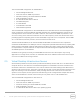
6 Virtual Desktop Infrastructure (VDI) A PowerEdge R730 VDI server was included in the reference system configured as previously described in Section 2.5. In order to evaluate the VDI server, NICE EnginFrame and Desktop Cloud Visualization (DCV) were installed on the reference system. The NICE EnginFrame and DCV solution provides remote visualization software and a grid portal for managing remote visualization sessions and HPC job submission, control, and monitoring.
Figure 47 NICE EnginFrame VIEWS Portal Figure 48 LS-PrePost with ODB-10M 51 Dell HPC System for Manufacturing—System Architecture and Application Performance
Figure 49 Fluent with small-indy Figure 50 mETA Post with motorbike 52 Dell HPC System for Manufacturing—System Architecture and Application Performance
One of the features of the NICE DCV Endstation client is the DCV Console. The console allows the user to dynamically adjust quality vs network bandwidth utilization by using a slider bar and to monitor the bandwidth being used by the client. For most uses, the 60% setting provides a good balance between bandwidth usage and image quality.
7 Conclusion This technical white paper presents a validated architecture for the Dell HPC System for Manufacturing. The detailed analysis of the building block configurations demonstrate that the system is architected for a specific purpose—to provide a comprehensive HPC solution for the manufacturing domain.