Analyzing Dell PS Series Storage with SAN Headquarters Dell Storage Engineering November 2019 A Dell Technical White Paper
Revisions Date Description September 2010 Initial release June 2010 Updated for SAN Headquarters v2.0 November 2010 Updated for SAN Headquarters v2.1 October 2015 Updated for SAN Headquarters v3.1 November 2019 vVols branding update THIS WHITE PAPER IS FOR INFORMATIONAL PURPOSES ONLY, AND MAY CONTAIN TYPOGRAPHICAL ERRORS AND TECHNICAL INACCURACIES. THE CONTENT IS PROVIDED AS IS, WITHOUT EXPRESS OR IMPLIED WARRANTIES OF ANY KIND. © 2010-2019 Dell Inc. All rights reserved.
Table of contents Revisions ............................................................................................................................................................................................... 2 Executive summary .............................................................................................................................................................................. 5 Acknowledgements ..............................................................................
3.3 Example 3: SQL application load example ........................................................................................................................ 41 3.3.1 Example 3 - SQL application load: Conclusion .................................................................................................................. 43 Example 4: Benchmark of Exchange ................................................................................................................................. 44 3.
Executive summary The purpose of this document is to help storage administrators and other IT professionals use SAN Headquarters to monitor PS Series SANs. Real-world examples are used to provide performance-analysis techniques and methods. SAN Headquarters provides exhaustive monitoring for performance and health of the PS Series groups. In addition, enhanced automation allows for proactive collection of diagnostic information for Dell™ support analysis and problem resolution.
1 SAN Headquarters overview SAN Headquarters (SAN HQ) is a client/server application that runs on Microsoft® Windows Server®. It monitors one or more PS Series groups and uses SNMP to query the groups. SAN HQ collects data over time and stores it on the server for retrieval and analysis. The client connects to the SAN HQ server, formats and displays the data in the graphical user interface (GUI).
Analysis • • • • • • • • • • • Determine how the group is performing, relative to a typical I/O workload of small, random I/O operations. This information helps determine if a group has reached its full capabilities, or whether the group workload can be increased without impacting performance. Allocate group resources more effectively by identifying underutilized resources.
1.1 SAN HQ architecture SAN HQ uses a client/server model which includes: SAN HQ Server: This is the server which runs the Monitor (EQLxPerf) service and communicates to the PS Series groups. SNMP requests are issued to collect configuration, status, and performance data. In addition, a syslog server may be configured to log hardware alarms or performance alerts (syslog is typically the same IP as the SAN HQ server and is configured in the PS Series Group Manager CLI or GUI).
Element Description To obtain a data point, the Monitor Service averages the data from consecutive polling operations. After a year (by default), the SAN HQ Server overwrites the oldest data. 3 Each computer running a Monitor Client accesses the log files maintained by the Monitor Service and displays the group data in the SAN HQ GUI. Note: The computer running the Monitor Service also has a Monitor Client installed. 1.
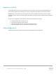
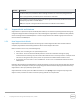
Figure 2 10 SupportAssist components and process Element Description 1 PS Series group at Site A (blue) and Site B (green) 2 PS Series SAN arrays 3 SAN networks (orange) 4 LAN networks (purple) 5 SAN HQ servers 6 SAN HQ clients 7 SSL Internet links 8 Internet 9 Secure SupportAssist web server Analyzing Dell PS Series Storage with SAN Headquarters | TR1050
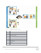
Element Description 10 Dell data center firewall 11 Dell Support and other departments 1.3 Information provided by SAN HQ 1.3.1 All Groups Summaries SAN HQ allows for monitoring of multiple PS Series arrays and provides summary information across all the groups monitored (Figure 3). To view this information, click All Groups Summary in the Servers and Groups tree.
1.3.2 Group information Once an individual group is selected, the informational dashboards shown in Figure 4 are available: Figure 4 Available functions by PS Series group Details for each selection are provided in the document, Dell EqualLogic SAN Headquarters Version 3.1 Installation and User’s Guide, available on eqlsupport.dell.com (login required). This document focuses on several panels to illustrate methods for analyzing PS Series data. 1.
Normally, each SAN HQ Client connects to the monitoring service to obtain and format the latest group performance data. Archiving the data allows you to analyze data when the SAN HQ monitoring service cannot be accessed. For example, if you start SAN HQ, but do not have access to the monitoring service, simply choose Ignore when launching SAN HQ, as shown in Figure 5. This allows SAN HQ to start in offline mode and then import archive files. Figure 5 1.5.
2 Using SAN HQ to find performance bottlenecks SAN HQ is designed to help identify hardware bottlenecks within the PS Series infrastructure. Many factors should be considered when troubleshooting or isolating the root cause. Hardware issues or misconfigurations should be identified and eliminated first. The Dell Storage PS Series is well suited for highly virtualized iSCSI connected environments. Configure the network according to Dell best practices for PS Series iSCSI networks.
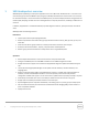
Applications Memory CPU NanoSeconds (ns) Data Request Millisecond (ms) < Milliseconds (ms) Microseconds (µsecs) Spinning Disks Figure 7 SSDs When observing latency relationships between components, DDR memory is much faster than spinning disks Looking at the previous figure, all resources should be understood from a utilization perspective. If the server has saturated processors or memory, latency suffers overall.
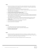
Figure 8 Performance and monitoring relationships: SAN HQ monitors iSCSI SAN for PS Series groups SAN HQ provides the resources needed to monitor and determine where bottlenecks may occur in the PS Series infrastructure. Server resources attached to the SAN such as processor and memory consumption may be understood using other tools such as Dell Performance Analysis Collection Kit (DPACK), Windows Perfmon, Linux iostat, or Dell’s Foglight. 2.
• • • 2.4 Throughput: Typically measured in megabytes per second (MB/s), this is the amount of bandwidth needed for the application. This may be derived by multiplying the I/O size by the number of IOPS. Understanding saturation points at the port level is important for high bandwidth needs. Queue depth: Indicates the number of requests that are lined up waiting on processing. Latency: The amount of time a request takes to arrive at the application.
10Gbps iSCSI networks are capable of accommodating typical bandwidth requirements. The PS Series architecture effectively aggregates all the ports to address additional throughput needs. 2.4.3 Servers The server should be eliminated as the source of a performance issue from a memory or processor perspective. Although spinning disk access is much slower than memory access speeds, other factors that are non-disk-related still need to be ruled out.
Table 1 General guidelines for IOPS per disk Disk type Random IOPS per disk (8KB I/O size) 7.2K NLSAS 75-90 10K SAS 130-185 15K SAS 180-210 SSD Depends on I/O size Reads/Writes disk manufacture and model I/O per disk is dependent on many factors such as speed, interface, disk classification (enterprise or consumer), as well as the distribution across each individual drive. Although Table 1 is a good reference, care should be taken into consideration that the table is not used as an absolute.
Figure 9 The sample period is from 06:00 to 13:00, while the summary (General Information) average is from the single interval selected (08:13) To find sample ranges for these averages, drag the mouse while clicking on the chart. To view information about the interval period in a pop-up window, hover the mouse over any point in time on the graph. Both of these techniques are demonstrated in Figure 10.
Figure 10 The interval span shows an average of all metrics over a span of an hour. Each interval in that span represents a sample of 15 minutes and 43 seconds. The range between 08:06 and 09:04 is averaged for the data in the table below the chart. If no range is selected, only that interval's average is displayed in the table. Note: It is important to understand the context for the averages of the polling periods as well as the sample intervals when reviewing SAN HQ.
3 Troubleshooting examples Troubleshooting SAN issues using SAN HQ is easily demonstrated using examples. This section includes several issues with possible resolutions. 3.
3.1.1 Example 1: Before Performance concerns are easily identified from the Combined Graphs dashboard where overall performance, capacity and trends are included in the display. For instance, if free capacity trends downward, then the focus on the volumes or snapshots consuming the most space. If latency were high in relation to the application tolerance, understanding which pools the members or volumes are taking the most resources from would be important.
Observations: Latency is above 25ms. Total IOPS are shy of 3000 from the host, capacity and total iSCSI sessions are ok. 3.1.1.1 Hardware and firmware details For a more thorough understanding of the array configuration, the Hardware/Firmware panel provides details. In this example, the Hardware/Firmware panel shows that two members each in their own pool. The default pool is in a RAID 6 configuration and contains a PS6210E with 7.2K 4TB NLSAS drives.
Figure 14 Experimental analysis of the group. The average IOPS is slightly over the estimated max IOPs. The Experimental Analysis defaults to the Group I/O view. The Hardware/Firmware displayed two pools that have to be selected individually to view the current I/O and the estimated maximum IOPS. When the group is selected, IOPS are only about 6% over the estimated maximum. If the I/O load could be more evenly spread out, the latency may be reduced for certain volumes.
In the Experimental Analysis panel, select the default pool to further expose the issues. Figure 15 Experimental analysis of the default pool The default pool shows that the current average IOPS far exceed the estimated maximum IOPS by 3.4 times. Latency is approximately 35ms for reads when observing this single pool. In this example, only the default pool has volumes allocated. The FASTPOOL15K is also a RAID 6 PS Series member however, it currently has no I/O as expected and shown below.
Figure 16 FASTPOOL15K Experimental Analysis panel. Currently no IOPs to this pool. When the Experimental Analysis panel displays the estimated maximum IOPS at the group, both pools are be included in the averages for the performance metrics. The average includes the potential of both pools regardless of any actual I/O occurring. This is important to understand when observing the Experimental Analysis tool.
3.1.1.3 Disks The Disk panel shows the individual IOPS for each disk, providing clues to the I/O profile. Under normal operations, the expected I/O rate from each disk is displayed. Disks that are over the expected IOPS, have high latency and queue depth reveal an over utilization. Table 2 shows that the expected IOPS for each disk in the NLSAS drives is approximately 85 IOPS/disk. The table data below the graph below shows that the IOPS/disk have exceeded this rule of thumb. Figure 17 28 7.
The disks in Figure 17 are 7.2K 4TB NLSAS disk, which typically are considered 100% utilized at 85 IOPS/disk. The Queue Depth on each disk is also indicating that disks may be waiting on results. A typical best practice is to keep the average disk queue depth below 10. Note: The table is only showing the averages for the selected time (7/1/2015 at 13:15). The graph will represent the host IOPS while the table data shows the metrics to each individual disk.
3.1.1.4 Conclusions for Example 1 – Over utilized pool This default pool is over utilized based on the latency, observations from the Experimental Analysis and the fact that the IOPS/Disk value exceeds the rule of thumb threshold. From these observations, it can be concluded that the capabilities of these drives have been exceeded. Two options can be explored for correcting the situation: • • 3.1.
Figure 18 All volumes on Pool. Notice the table data showing highest IOPS by volume. FASTPOOLXV contains a single PS6210XV in a RAID 6 configuration. Since this pool has a single member with 15K 146GB SAS drives, available capacity should be considered before moving. The SAN HQ Capacity panel displays the overall capacity of the default pool as indicated in Figure 19.
Figure 19 Capacity for FASTPOOL15K shows 2.42TB of free space Since these are small volumes (100GB each), the volumes can be safely moved to the destination pool. The Group Manager GUI prevents the move if space is not available. For this example, analyzing the individual volume capacity is not necessary since the entire space in use of the default pool is well below the free space in the FASTPOOL15 pool. 3.1.2.
Figure 20 3.1.3 Volumes split between the default and the FASTPOOL15K in the Group Manager GUI Example 1: After volumes are moved After the volumes completed the move, the same performance test was run again to show the improvement. The following graphs from the I/O panel show the improved latency as well as additional IOPS achieved by splitting the volumes into the two pools.
Figure 21 Group view from the I/O panel showing the results of moving the volumes The arrows in Figure 21 indicate the improvement made after moving the volumes to the new pool. The increase in IOPS indicates that the pool had pent-up demand which was relieved by moving the volumes to the pool with faster drives. In addition, a lower latency was achieved even with the higher I/O load.
Figure 22 3.1.3.1 Volume IOPS distribution after the move showing more I/O activity to the FASTPOOL15K Iterative process of moving volumes Manually moving volumes to another pool is a technique which allows for appropriate placement of workloads based on I/O characteristics or business importance. This methodology may be an iterative process and to fully even the load, several volume moves may need to be considered to balance the workload to the desired goal.
Figure 23 3.1.3.2 After the second volume move, the IOPS favor the faster pool. Example 1 Move: Conclusion This example demonstrated a method of associating the faster member to the higher workload. First, a few volumes were moved and the activity monitored. As a result, the decision was made to move the volumes again according to their new workload profile.
3.1.4 Example 1: After merging pools Merging the two pools simply allows the PS Series to virtualize all of the volumes across the aggregate spindles. The PS Series will move data appropriately based on capacity between the resulting members. Typically, this is the simplest method. Notice the results are similar to moving the volumes to separate pools. Figure 24 3.1.4.1 Results after merging the two pools. Latency is below 20ms and IOPS increased to over 7000.
into a single pool simplifies administration and allows the array to optimize for performance and capacity. Both methods have their merits and typically achieve very similar performance results.
3.2 Example 2: Performance planning As a storage administrator, planning for new workloads and correcting bottlenecks are frequent tasks. This next example will demonstrate how a solution may be designed to adequately plan and correct bottlenecks. In this situation, the first example of the over utilized pool is used to determine the best solution for fixing the performance issues. First, the Experimental Analysis panel is used to indicate how many more IOPS are needed. 3.2.1.
The “write penalty” is the additional IOPS needed to protect the disks with RAID. Table 3 shows the values for the available RAID policies for PS Series arrays. Table 3 Write Penalty based on RAID RAID Policy Write Penalty RAID 10 2 RAID 50 4 RAID 6 6 Note: RAID Policy is defined on the PS Series member. The Pool may have multiple members at different RAID policies. For this example, a RAID 6 solution will be considered which has a write penalty of 6. Plugging in .7 to represent the reads and .
3.2.1.3 Example 2 - Performance planning: Conclusion A new PS6210XV will have 24x15K disks and should be added to the group. The new member would handle the current IOPS. However, the pent-up demand may indicate an additional member may need to be added to the pool. This sizing methodology should be useful to help properly design a solution to meet the desired performance requirements. 3.3 Example 3: SQL application load example For an application-relevant example, consider a Microsoft SQL load process.
Actual IOPS > MAX Latency looks good Figure 27 SQL Insert commands loading tables show IOPS exceed the estimated maximum IOPS, however performing with low latency From the Experimental Analysis panel, the overall I/O load appears to indicate that this PS Series group is exceeding its capabilities. However, latency is below 15ms. For this part of the application 15ms latency is acceptable. The actual pressure on the disks should also be verified by clicking Hardware / Firmware > Disks as shown below.
Figure 28 3.3.1 Disk table data Example 3 - SQL application load: Conclusion Although the Experimental Analysis seems to indicate that the maximum capabilities of this array are being exceeded, the actual workload latency and disk IOPS are within acceptable performance criteria. One of the goals of this example is to show the importance of understanding that the estimated maximum IOPS should be used as a tool and validated by reviewing latency and actual disk IOPS measurements.
3.4 Example 4: Benchmark of Exchange This example is from a Microsoft Exchange Solution Review Program (ESRP). From an analysis perspective, we want to see how well the PS Series array handles a large mailbox configuration. This test typically pushes the limits of the resources to show maximum efficiencies for the underlying solution. The Combined Graphs show very distinct I/O patterns. One part of the I/O is significantly lower than the other. Latency also appears very high for most of the sample.
Figure 30 Experimental Analysis shows latency below 14ms, steady IOPS of 900 and plenty of headroom from estimated maximum IOPS The adjusted view provides a more accurate overview of the I/O load, and indicates a successful test. Also important is the length of an interval period considered for the averages. The interval for each sample in this example is over six minutes. If more granularity is needed, SAN HQ provides this with the Live View tool demonstrated in the next example.
3.5 Example 5: Live View Live View allows for up to a 10-minute sample at one-second intervals. More precise sample intervals helps in difficult troubleshooting scenarios, planning for new applications or just establishing a baseline profile of an existing application. Live View sessions may also be saved for later analysis.
This Live View sample shows I/O spikes of over 1000 and a few latency spikes. The latency spikes correspond to larger I/O sizes (as expected). In this case, Live View is providing a more detailed picture of the ESRP I/O profile. Although the spikey behavior when shorter intervals are measured is evident, this does not necessarily represent a problem. More accurately, these spikes should be considered when sizing to solutions close to the maximum capabilities of the array. 3.
The example below shows a situation where choosing the more reliable RAID policy has little impact on the current IOPS. The difference between the current IOPS and the possible maximum IOPS allows for headroom even considering the maximum IOPS for RAID 6 will be less than the RAID 50 policy. Figure 34 3.
Figure 35 Disk performance on the hybrid showing the SSDs performing around < 4000 IOPS while the NLSAS is near 76 IOPS The table below the chart shows the SSDs in excess of 3800 IOPS while the 7.2K SAS drives are near 75 IOPS per disk. SAN HQ can be used here to view the placement of data in relation to the I/O needs. In the I/O panel, Group I/O Load Space Distribution data is represented according to its frequency of access to the hybrid.
High Medium Low Figure 36 Group I/O Load Space Distribution indicates around 62GB are high load pages, 6GB are medium load pages and over 100TB are consider low load The I/O panel displays the breakdown of high, medium and low load distribution. In this example, the highest load needs are about 60GB of space and that is accounted for on the SSD drives. However, medium and low loads may also exist on the SSDs; these may be moved to the 7.
3.8 Example 8: VMware vSphere Virtual Volumes Starting with ESX 6.0, a new feature is available with VMware® vSphere® known as Virtual Volumes, or vVols. This feature is supported on PS Series firmware version 8 and later and SAN Headquarters 3.1 and later. vVols are different from the traditional PS Series volumes and have their own views to show capacity and performance. Information about SAN HQ vVols: • • • • • Volumes are not associated with vVols they are a separate object type.
Figure 38 52 vVol capacity shown in the All Groups Summaries > Volume Capacity Summary Analyzing Dell PS Series Storage with SAN Headquarters | TR1050
• View vVol performance by selecting Group, Pool, Member, Storage Container, VMs or VVols menu options. In Figure 39, performance metrics are demonstrated for the storage container “test” (which is on this array).
4 Summary SAN HQ acts like an in-flight data recorder for your PS Series group that is a powerful monitoring and analysis tool. It provides SAN administrators with valuable insight into the health of their storage environment. The easy-to-use graphical interface provides information on PS Series group capacity, I/O performance, network data, member hardware and configuration, and volume data.
A SAN Headquarters tips and techniques Several practices are helpful for day to day monitoring of the PS Series environment with SAN HQ. The following tips are for reference. A.1 Creating SAN HQ archives Over time, SAN HQ automatically compresses the time for each interval to save log space. Archives are one way to capture the more granular interval periods.
B Additional resources Dell.com/support is focused on meeting your needs with proven services and support.