Manual EN – Version 2.
Table of Contents 1 2 3 Indications for Use.......................................................................................................... 4 1.1 Symbols .................................................................................................................. 4 1.2 Safety ...................................................................................................................... 4 1.3 Warning................................................................................
5.3 Repeater Table ......................................................................................................52 5.3.1 6 Table Fields ....................................................................................................52 Administration View .......................................................................................................53 6.1 Current Project Settings .........................................................................................54 6.1.
1 Indications for Use It is essential to read the operating instructions carefully and completely before using the first time the equipment and software. They contain important information on safety, installation and use. Keep these instructions in a safe place. 1.1 Symbols Warning of dangerous situations that can cause injury and damage to the devices. Warning The ZONESCAN Correlating Radio Noise Data Logger contains a very powerful magnet.
battery, please contact your Gutermann distributor. If you use the software and associated mobile equipment, pay the necessary attention particularly in traffic. 1.3 Warning The ZONESCAN Correlating Radio Noise Data Logger contains a very powerful magnet. The operation of cardiac pacemakers and implanted defibrillators can be influenced. People with cardiac pacemakers and implanted defibrillators are not permitted anywhere near this product. ZONESCAN S-Alpha does emit electromagnetic fields in operation.
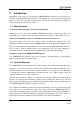
2 Introduction Gutermann Technology has developed the ZONESCAN NET System for professional leak detection in public drinking water pipelines. This unmanned, acoustic leak monitoring system with noise level and correlation measurements ensures that leak detection specialists are deployed only at the actual leak locations. 2.
Figure 1: Functionality of logger, repeater and alpha Interactive communication between ZONESCAN NET and the leak detector While conventional radio loggers are equipped with a simple radio transmitter, the ZONESCAN Correlating Radio Noise Data Loggers feature a transceiver (combined transmitter and receiver). This allows for interactive communication between the sensor located in the chamber and the leak detector.
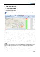
3 Leak Detection View 3.1 Leak Detection Map 3.1.1 Structure of the Screen Note! If the alpha fails, no data can be collected by the repeater and the logger and transmitted Figure 2: Structure of the screen with numbers to for explanation Map Area The Map Area contains a map by Google Maps with the area of the selected project. Use the buttons located above the map to execute various functions which vary depending on "View" - Leak Detection or Maintenance.
The measurement period can be changed in the drop-down menu. Select from 5 days, 30 days or an entire month. The current setting is displayed at the right. Selected Item Use the blue arrow buttons to change between the individual values in the list area. The current selection is displayed in the upper area. List Area In List area, the user finds all data relevant for the evaluation. Logout Button The user logs out with the logout button.
3.1.
Zoom all items which adjusts the map by automatically to fit zooming in or out to fit all items in the window Shows or hides the map legends at the bottom of the screen Displays the logger numbers or not – next to the colored dots representing the loggers Displays the logger noise levels in dB (decibel) – on top of the colored dots Figure 5: In the top left corner all four symbols are explained in speech bubbles 11 I 72
Figure 6: Zoom In/Out The Google Maps Zoom Slider allows one to zoom in or out Google Street View This powerful function that Google Maps have introduced allows the user to view and walk through the photographed 3D streets. If there is an orange Pegman present above the zoom bar then Google Street View is available. Follow the link for further detail about using Google Street View: https://support.google.
Figure 8: Google Street View Pegman (red circle) • Hover the cursor over the orange Pegman and he will lean forward as shown above Figure 9: Google Street View moving the Pegman (red circle) • Click and hold the cursor on the person then drag him to a chosen location on the street which will highlight blue to show which streets have the street view present.
Figure 10: Google Street View 1st person perspective • The map changes to a photographic image of the street with the ZONESCAN Logger plotted in in place.
Figure 11: Google Street View 1st person perspective – cont. • The user is able to turn 360degrees on the spot by moving the cursor left or right until a rectangular white shadow appears, simply click the mouse to move in the chosen direction.
Figure 13: Google Street View Correlation Point (red circle) An orange fuzzy spot plotted on the road represents a correlated point for further investigation. This is a very powerful remote tool for the leakage technician to further investigate. 3.1.
• In the window above the Probable, Possible, w/o Pipe and Out of Bracket correlations maybe ticked to show or unticked to hide the correlation icons Figure 15: Logger Noise Drop-Down Menu • Shows the Logger Noise options Probable, Possible and No Leak, tick to display all the Loggers on the map or untick to hide any of the options Figure 16: Logger Custom Drop-Down Menu • Allows the user to select the pipe network created using the correlation wizard or KML (Keyhole Markup Language) layer provided by the
3.2 Correlations Table Figure 17: Correlated Leaks • The sorting of the tables can be changed at any time. Click the small arrow in the title field of the value that you would like to change. In the selection box that opens, you can sort in either alphabetical or reverse alphabetical orderThe columns can also be displayed or hidden from the table. To do this, click the small arrow in the title field. In the selection menu that appears, move the cursor to the Columns item.
Figure 18: Correlation Table Fields Quality A statement on the Quality of the correlation graph is made. The assessment ranges from 0 - 100%. The settings for the display of a possible or probable leak are made under Administration in Settings Logger 1 Reference number of the first Logger that was correlated Logger 2 Reference number of the second Logger that was correlated Distance L1 Distance L1 specifies the distance between Logger 1 and the noise source.
Pipe Length This is the total Pipe Length between Logger 1 and Logger 2 Pipe Setup Located in the Pipe Setup field are red, yellow or green indicators Red indicators indicate that no pipe settings have been entered yet and the used data were taken over from the default values Yellow images appear if manual settings were made and not all details are known (pipe length, diameter and material are known).
Figure 20: Entering pipe settings – cont. • Click the “Add Segment” button to enter a new pipe segment. Then complete the “Length, Material and Diameter” fields. The sound velocity is automatically calculated from your values and entered in the respective field.
Figure 21: Adjusting loggers • In the next step, you have the option of changing the course of the pipeline. To do this, click the small box in the middle of the pipe that you would like to move. With the mouse pressed down, drag the pipe to the desired position • You can now repeat this with the individual segments until the pipeline is correctly positioned. Use “Undo” to undo your last change.
Figure 22: Adjusting the pipeline • Next, you are prompted to edit the properties of the individual segments of the pipeline. Complete the “Length, Material and Diameter” fields Note! If the data – Length, Material and Diameter – are contained in a displayed KML (Keyhole Markup Language) layer, it can be displayed in the map by clicking the corresponding pipeline.
Figure 23: Adjusting the pipeline – Finish Note! It is possible that the Pipe Wizard calculation cannot be performed immediately. It depends on the complexity of the recalculations and the workload of the server 3.2.4 Correlation Context Menu • A context menu can be displayed for each individual, correlated leak. To do this, select the value in the table that you would like to visualize • Right-click to open the context menu. Here, you can select the type of graph to be displayed.
Figure 24: Context menu for correlations Show in Street View The map will switch to Google Street View and automatically zoom in on the chosen correlated point.
3.2.5 Correlation Graph Figure 26: Correlation Graph Correlation is a mathematical method for comparing two time synchronized signals with one another. A leakage noise is simultaneously recorded by two sensors at different locations which are represented by the black lines at either side of the graph if the pipe data is known. The sound emitted by the leak spreads in the water pipe at a defined sound velocity. If the acoustic event were to be brief and occur only once, e.g.
retroactively separating such interfering noise to better identify the correlation maximum caused by the leak. 3.2.6 Correlation Spectrum Figure 27 Correlation Spectrum The correlation spectrum is a combination of the signal spectra of the two sensors, which is used for the correlation on the pipeline between the two sensors. In these common spectra, it may be possible to identify the influence of noises not related to the leak (e.g., electrical noise or pumps) on the correlation result (see also 3.2.
3.2.7 Correlation Report Choose the required options by ticking the box opposite and then click open. A new window will open in the browser with the relevant maps and graphs associated with the chosen correlation.
Figure 30: Correlation Report – Part 2 29 I 72
3.3 Logger Noise Table Displayed in the Logger Noise Table are all values that are needed for an evaluation. Figure 31: Logger Noise Table 3.3.1 Table Fields Leak Score The Leak Score is specified in a range from 0 to 100. The higher the number, the greater the probability that measurements will actually detect a leak. The goal of the noise measurement with Loggers is to obtain as reliable a statement as possible regarding the presence of a leak at a specific point of the monitored water network.
(spectrum). These values are used, in particular, for removing background noise. The frequency spectrum data enables the algorithm to differentiate between leak noise and mechanical noises. In addition, if there is a correlation at the same position near the logger for more than one day, this will also increase the leak score. The result is output as the Leak Score in a range from 0 to 100.
3.3.2 Logger Noise Context Menu A context menu can be displayed for each Logger. To do this, select the Logger in the table that you would like to visualize. Right-click to open the context menu. Here, you can select the type of menu that is displayed. In addition, you can insert a comment. The same menu can be opened by right-clicking a Logger on the map.
Histogram The histogram is the graphical display of a noise distribution of the measured sound level Figure 34: Logger Histogram 33 I 72
Histogram cont. During noise monitoring, the noise level is repeatedly measured in intervals of a few seconds. During a one-hour measurement period (e.g., from 2 a.m. to 3 a.m.), several hundred individual measurement values are collected. The sound level is measured in dB. If, for example, the sound intensity of 15 dB is measured 120 times, this sound intensity has a frequency value of 120. Other sound intensity values are measured with a different frequency.
In figure 37, you see a typical spectrum of a leakage noise. It is clearly seen that the curve differs from that of a spectrum with electrical influence.
Leak Score History The Leak Score History visualizes the historical values from the last 30 days, 3 months, 6 months, 12 months, 2 years or full history as long as the data is available for the time span. If the data available is less than a chosen period then the software will adjust the window to fit. On days with sound signal, the leak score is shown in blue, otherwise in green.
Figure 38: Logger dBmin History Play Noise The actual leak noise sample can be played through the PC speakers or headphones to help identify the type of sound recorded by the chosen logger. To help distinguish between background sound and leak sound compare a logger which has a leak score of 0 (zero) and then listen to a logger with a high leak score • Depending on your browser, either click the Signal Spectrum and choose the Download Sound File or press the “Play” button.