Expand Configuration and Management Manual (H06.03+)

Tuning
Expand Configuration and Management Manual—529522-002
19-32
Example 2: Reducing Passthrough Traffic
Notice that the source and destination of passthrough traffic cannot be identified from
Measure data.
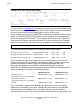
By comparing the total DIRECT frames to the total FORWARD frames, you can
determine that \JUICE is used primarily as a switch in the network among \TOPPER,
\TONY, and \TRGGR. Ninety-seven percent of the data (1,184,392 frames, as shown
in the TOTAL FORWARD column) sent to \JUICE from \TOPPER was passed on to
other nodes.
Similar measurements made on \TOPPER and \TONY would show that all the frames
forwarded through \JUICE to and from \TONY went to \TOPPER. About 300,000 bytes
were received from \TONY and sent to \TOPPER, and about 300,000 bytes were
received from \TOPPER and sent to \TONY. As a result, \JUICE is spending more time
processing passthrough traffic between \TOPPER and \TONY than it is sending direct
traffic.
Making a direct connection between \TONY and \TOPPER would eliminate 600,000
frames of passthrough traffic on \JUICE and would result in a 40 percent reduction in
unnecessary switched traffic. Additional benefits would include a reduction in the
number of processors, communications devices, and communications links used on
\JUICE as well as in the network.
Measuring Passthrough Traffic in an Entire Network
Example 19-8 shows another step in the complete analysis of passthrough traffic in an
Expand network. In this example, data taken from SCF is used to compute the total
network overhead of passthrough traffic for each source and destination at one node.
This single-node analysis could be extended to all nodes in a network.
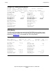
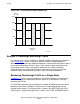
Example 19-7. Passthrough Traffic From Measure SYSTEM Counters on \JUICE
<========Expand FRAMES============> TOTAL TOTAL
SYSTEM LINKS SENT RECEIVED SENT-FWD RCVD-FWD DIRECT FORWARD
===================================================================
\TOPPER 9816 21605 20549 604067 580325 42154 1184392
\TONY 98328 292025 386625 294042 310158 678650 604200
\TRIGGR 46 177 140 123022 85795 317 208817
\SCOUT 24779 51396 55189 102819 2160 106585 104979
\FURY 10529 21725 23774 50291 50734 45499 101025
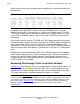
Note. The table in Example 19-8 was prepared by combining information from Expand
subsystem SCF PATH STATS and PROBE commands and then manipulating the data with a
spreadsheet. The STATS command showed the traffic, while the PROBE command showed
the number of hops. Example 19-8
is an illustration of one simple technique for deriving a
thorough understanding of network performance from standard, readily available
instrumentation.