
Guardian Programmer's Guide
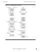

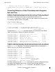
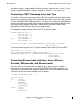
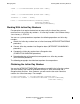
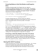
Table Of Contents
- Guardian Programmer’s Guide
- Contents
- What’s New in This Manual
- About This Manual
- Legal Notices
- 1 Introduction to Guardian Programming
- 2 Using the File System
- 3 Coordinating Concurrent File Access
- 4 Using Nowait Input/Output
- 5 Communicating With Disk Files
- Types of Disk Files
- Using Unstructured Files
- Creating Unstructured Files
- Opening Unstructured Files
- Positioning, Reading, and Writing With Unstructured Files
- Locking With Unstructured Files
- Renaming Unstructured Files
- Avoiding Unnecessary Cache Flushes to Unstructured Files
- Closing Unstructured Files
- Purging Unstructured Files
- Altering Unstructured-File Attributes
- Using Relative Files
- Using Entry-Sequenced Files
- Using Key-Sequenced Files
- Creating Key-Sequenced Files
- Opening Key-Sequenced Files
- Positioning, Reading, and Writing With Key-Sequenced Files
- Locking, Renaming, Caching, Closing, Purging, and Altering Key-Sequenced Files
- Key-Sequenced File Programming Example
- Using Alternate Keys With an Entry-Sequenced File
- Using Alternate Keys With a Key-Sequenced File
- Using Partitioned Files
- Using Alternate Keys
- 6 Communicating With Processes
- Sending and Receiving Messages: An Introduction
- Sending Messages to Other Processes
- Queuing Messages on $RECEIVE
- Receiving and Replying to Messages From Other Processes
- Receiving Messages From Other Processes: One-Way Communication
- Handling Multiple Messages Concurrently
- Checking for Canceled Messages
- Receiving and Processing System Messages
- Handling Errors
- Communicating With Processes: Sample Programs
- 7 Using DEFINEs
- 8 Communicating With a TACL Process
- 9 Communicating With Devices
- 10 Communicating With Terminals
- 11 Communicating With Printers
- 12 Communicating With Magnetic Tape
- Accessing Magnetic Tape: An Introduction
- Positioning the Tape
- Reading and Writing Tape Records
- Blocking Tape Records
- Working in Buffered Mode
- Working With Standard Labeled Tapes
- Enabling Labeled Tape Processing
- Creating Labeled Tapes
- Checking for Labeled Tape Support
- Accessing Labeled Tapes
- Writing to the Only File on a Labeled Tape Volume
- Writing to a File on a Multiple-File Labeled Tape Volume
- Writing to a File on Multiple Labeled Tape Volumes
- Reading From the Only File on a Labeled Tape Volume
- Reading From a File on a Multiple-File Labeled Tape Volume
- Reading From a File on Multiple Labeled Tape Volumes
- Accessing a Labeled Tape File: An Example
- Working With Unlabeled Tapes
- Terminating Tape Access
- Recovering From Errors
- Accessing an Unlabeled Tape File: An Example
- 13 Manipulating File Names
- 14 Using the IOEdit Procedures
- 15 Using the Sequential Input/Output Procedures
- An Introduction to the SIO Procedures
- Initializing SIO Files Using TAL or pTAL DEFINEs
- Opening and Creating SIO Files
- Getting Information About SIO Files
- Reading and Writing SIO Files
- Accessing EDIT Files
- Handling Nowait I/O
- Handling Interprocess Messages
- Handling System Messages
- Handling BREAK Ownership
- Handling SIO Errors
- Closing SIO Files
- Initializing SIO Files Without TAL or pTAL DEFINEs
- Using the SIO Procedures: An Example
- 16 Creating and Managing Processes
- 17 Managing Memory
- An Introduction to Memory-Management Procedures
- Managing the User Data Areas
- Using (Extended) Data Segments
- Overview of Selectable Segments
- Overview of Flat Segments
- Which Type of Segment Should You Use?
- Using Selectable Segments in TNS Processes
- Accessing Data in Extended Data Segments
- Attributes of Extended Data Segments
- Allocating Extended Data Segments
- Checking Whether an Extended Data Segment Is Selectable or Flat
- Making a Selectable Segment Current
- Referencing Data in an Extended Data Segment
- Checking the Size of an Extended Data Segment
- Changing the Size of an Extended Data Segment
- Transferring Data Between an Extended Data Segment and a File
- Moving Data Between Extended Data Segments
- Checking Address Limits of an Extended Data Segment
- Sharing an Extended Data Segment
- Determining the Starting Address of a Flat Segment
- Deallocating an Extended Data Segment
- Using Memory Pools
- 18 Managing Time
- 19 Formatting and Manipulating Character Data
- Using the Formatter
- Manipulating Character Strings
- Programming With Multibyte Character Sets
- Checking for Multibyte Character-Set Support
- Determining the Default Character Set
- Analyzing a Multibyte Character String
- Dealing With Fragments of Multibyte Characters
- Handling Multibyte Blank Characters
- Determining the Character Size of a Multibyte Character Set
- Case Shifting With Multibyte Characters
- Testing for Special Symbols
- Sample Program
- 20 Interfacing With the ERROR Program
- 21 Writing a Requester Program
- 22 Writing a Server Program
- 23 Writing a Command-Interpreter Monitor ($CMON)
- Communicating With TACL Processes
- Controlling the Configuration of a TACL Process
- Controlling Logon and Logoff
- Controlling Passwords
- Controlling Process Creation
- Controlling Change of Process Priority
- Controlling Adding and Deleting Users
- Controlling $CMON While the System Is Running
- Writing a $CMON Program: An Example
- Debugging a TACL Monitor ($CMON)
- 24 Writing a Terminal Simulator
- 25 Debugging, Trap Handling, and Signal Handling
- 26 Synchronizing Processes
- 27 Fault-Tolerant Programming in C
- Overview of Active Backup Programming
- Summary of Active Backup Processing
- What the Programmer Must Do
- C Extensions That Support Active Backup Programming
- Starting the Backup Process
- Opening a File With a Specified Sync Depth
- Retrieving File Open State Information in the Primary Process
- Opening Files in the Backup Process
- Retrieving File State Information in the Primary Process
- Updating File State Information in the Backup Process
- Terminating the Primary and Backup Processes
- Organizing an Active Backup Program
- Updating State Information
- Providing Communication Between the Primary and Backup Processes
- Programming Considerations
- Comparison of Active Backup and Passive Backup
- Active Backup Example 1
- Active Backup Example 2
- 28 Using Floating-Point Formats
- Differences Between Tandem and IEEE Floating-Point Formats
- Building and Running IEEE Floating-Point Programs
- Compiling and Linking Floating-Point Programs
- Link-Time Consistency Checking
- Run-Time Consistency Checking
- Run-Time Support
- Debugging Options
- Conversion Routines
- Floating-Point Operating Mode Routines
- A Mixed Data Model Programming
- Glossary
- Index

Managing Time
Guardian Programmer’s Guide — 421922-014
18 - 8
Working With 64-Bit Julian Timestamps
TYPE := SINCE^COLD^LOAD;
TIME1 := JULIANTIMESTAMP(TYPE);
.
.
TYPE := SINCE^COLD^LOAD;
TIME2 := JULIANTIMESTAMP(TYPE);
INTERVAL := TIME2 - TIME1;
Obtaining a Julian Timestamp: Remote Node
If you are dealing with timestamps on a remote node, then the relevant Julian
timestamp is the one that is generated on that node. This is because system time on
the remote node may be different from system time on the local node; the operating
system makes no attempt to synchronize clocks between nodes.
If, for example, you want to know how much time has passed since a specific file on a
remote node was last updated, you would find out using the last update timestamp on
the file and the current timestamp from the remote node.
When establishing the current time on a remote node, you should attempt to
compensate for the time it takes to send the message containing the timestamp to the
local node. You find this out using the following sequence:
1. Call the JULIANTIMESTAMP procedure for the local node to return the number of
microseconds since cold load.
2. Call the JULIANTIMESTAMP procedure for the remote node.
3. Call the JULIANTIMESTAMP procedure for the local node to return the number of
microseconds since cold load.
4. Compute the difference between the timestamps returned in Steps 1 and 3. This is
the time taken to send a message from the local node to the remote node and then
to send a message back to the local node from the remote node.
5. Divide the time delay indicated in Step 4 by 2 to get the time to send a message in
one direction.
6. Add the delay indicated in Step 5 to the remote timestamp returned in Step 2. The
result is a current timestamp for the remote node.
The following example calculates the time since the last update of a file named DFILE
on a remote node named \SYS2.
LITERAL GET^TIME^OF^LAST^UPDATE = 144,
CURRENT^GMT = 0,
SINCE^COLD^LOAD = 3;
INT .RESULT[0:3],
Note. The above algorithm yields an approximate result. The error in the result can be as
large as the value computed in Step 5.