HP NonStop SQL/MX Query Guide Abstract This guide describes how to understand query execution plans and write optimal queries for an HP NonStop™ SQL/MX database. It is intended for database administrators and application developers who use SQL/MX to query an SQL/MX database and who have a particular interest in issues related to query performance. Product Version NonStop SQL/MX Releases 2.0 and 2.1 Supported Release Version Updates (RVUs) This publication supports G06.
Document History Part Number Product Version Published 429856-001 NonStop SQL/MX Release 1.5 November 2001 522677-001 NonStop SQL/MX Release 1.8 December 2002 523728-001 NonStop SQL/MX Release 2.0 April 2004 523728-002 NonStop SQL/MX Release 2.0 August 2004 523728-003 NonStop SQL/MX Releases 2.0 and 2.
HP NonStop SQL/MX Query Guide Index Examples What’s New in This Manual vii Manual Information vii New and Changed Information Figures Tables vii About This Manual ix Audience ix Organization ix Related Documentation x Notation Conventions xii 1.
2. Accessing SQL/MX Data (continued) Contents 2. Accessing SQL/MX Data (continued) Controlling the Number of Key Columns Used by MDAM MDAM’s Use of DENSE and SPARSE Algorithms 2-17 2-17 3.
. Forcing Execution Plans (continued) Contents 5.
Contents 7. Operators and Operator Groups (continued) 7.
. Operators and Operator Groups (continued) Contents 7. Operators and Operator Groups (continued) SPLIT_TOP Operator 7-49 SUBSET_DELETE Operator 7-50 SUBSET_UPDATE Operator 7-51 TRANSPOSE Operator 7-52 TUPLE_FLOW Operator 7-52 TUPLELIST Operator 7-53 UNIQUE_DELETE Operator 7-53 UNIQUE_UPDATE Operator 7-55 UNPACK Operator 7-56 VALUES Operator 7-57 8.
Examples Contents Examples Example 1-1. OR Optimization DDL 1-13 Figures Figure 1-1. Figure 4-1. Figure 4-2. Figure 5-1. Figure 5-2. Figure 5-3. Figure 5-4. Figure 5-5. Figure 5-6. Figure 5-7. Figure 8-1. Figure 8-2. Figure 8-3. Figure 8-4. Figure 8-5. Figure 8-6. Figure 8-7. Figure 8-8.
What’s New in This Manual Manual Information HP NonStop SQL/MX Query Guide Abstract This guide describes how to understand query execution plans and write optimal queries for an HP NonStop™ SQL/MX database. It is intended for database administrators and application developers who use SQL/MX to query an SQL/MX database and who have a particular interest in issues related to query performance. Product Version NonStop SQL/MX Releases 2.0 and 2.
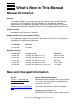
New and Changed Information What’s New in This Manual Section New or Changed Information Section 4, Reviewing Query Execution Plans Removed DETAILED_STATISTICS and PERTABLE statistics information as these features are not yet included in SQL/MX. Section 6, Query Plan Caching Corrected information regarding queries that are compiled repeatedly. Section 7, Operators and Operator Groups Clarified status of MATERIALIZE operator. Section 8, Parallelism Corrected description information.
About This Manual This guide describes the use and formulation of queries, how to understand query execution plans, and how to affect the performance of NonStop SQL/MX databases.
Related Documentation About This Manual Related Documentation This manual is part of the HP NonStop SQL/MX library of manuals, which includes: Introductory Guides SQL/MX Comparison Guide for SQL/MP Users Describes SQL differences between SQL/MP and SQL/MX. SQL/MX Quick Start Describes basic techniques for using SQL in the SQL/MX conversational interface (MXCI). Includes information about installing the sample database.
Related Documentation About This Manual SQL/MX Report Writer Guide Describes how to produce formatted reports using data from a NonStop SQL/MX database. SQL/MX Connectivity Service Manual Describes how to install and manage the SQL/MX Connectivity Service (MXCS), which enables applications developed for the Microsoft Open Database Connectivity (ODBC) application programming interface (API) and other connectivity APIs to use SQL/MX.
Notation Conventions About This Manual This figure shows the manuals in the SQL/MX library: Programming Manuals Introductory Guides SQL/MX Comparison Guide for SQL/MP Users SQL/MX Quick Start SQL/MX Programming Manual for C and COBOL SQL/MX Programming Manual for Java Reference Manuals SQL/MX Reference Manual SQL/MX Messages Manual SQL/MX Glossary SQL/MX Connectivity Service Administrative Command Reference DataLoader/MX Reference Manual Specialized Guides SQL/MX Installation and Management Gu
General Syntax Notation About This Manual This requirement is described under Backup DAM Volumes and Physical Disk Drives on page 3-2. General Syntax Notation The following list summarizes the notation conventions for syntax presentation in this manual. UPPERCASE LETTERS. Uppercase letters indicate keywords and reserved words; enter these items exactly as shown. Items not enclosed in brackets are required. For example: MAXATTACH lowercase italic letters.
General Syntax Notation About This Manual braces on each side of the list, or horizontally, enclosed in a pair of braces and separated by vertical lines. For example: LISTOPENS PROCESS { $appl-mgr-name } { $process-name } ALLOWSU { ON | OFF } | Vertical Line. A vertical line separates alternatives in a horizontal list that is enclosed in brackets or braces. For example: INSPECT { OFF | ON | SAVEABEND } … Ellipsis.
1 Compiling and Executing a Query Use the information in this section to understand how your queries are compiled and executed. • • How the Compiler Works on page 1-2 How the Executor Processes the Plan on page 1-14 Overview At the highest level, compiling and executing an SQL query with SQL/MX consists of two basic steps. 1. The SQL compiler processes the query and produces a query execution plan.
Compiling and Executing a Query • How the Compiler Works Modifying the database by adding columns to a table, splitting or merging partitions, and creating and dropping indexes. For more information, see Improving Query Performance on page 1-6. How the Compiler Works To compile a query, the SQL compiler needs information about the tables listed in the query and the query environment. The necessary table information is listed in the schema metadata tables from the SQL/MX catalog.
Parsing, Binding, and Normalizing Compiling and Executing a Query Parsing, Binding, and Normalizing The initial steps in the compile process—parsing, binding, and normalizing—prepare the query for the optimizer. Before query optimization begins, the query tree that is produced by the parser is bound with information from the metadata. Certain query processing instructions in addition to default values needed for optimizing the query are processed.
Parsing, Binding, and Normalizing Compiling and Executing a Query by the optimizer go into the search space, where they are stored in search memory. • Principle of Optimality In this strategy, the optimizer starts at the top of the normalized query tree and breaks the optimization tasks into smaller tasks (or subtasks). Depending on the physical properties of the operators, the optimizer combines the optimal solutions of the subtasks for the completed plan.
Query Plan Caching Compiling and Executing a Query is a physical operator. Recursive application of implementation rules result in a query execution plan that consists only of physical operators. Such plans or subplans can be executed by the executor because they have physical properties, and their cost can be estimated by the optimizer. The implementation rule phase refines the earlier rules that result in physical nodes.
Compiling and Executing a Query Improving Query Performance Two queries are considered equivalent for the purposes of caching if their canonical forms are the same.
Compiling and Executing a Query • • Improving Query Performance Canonical reorder of the tables in the query tree Constant folding. Constant folding is a compiler optimization technique where an expression, consisting only of constants, is evaluated at compile time. For example: WHERE AGE_IN_DAYS>(2005-1960)*365 When constant folded, this expression becomes WHERE AGE_IN_DAYS>16425. • Syntactic and semantic sort elimination In the optimizer, transformations are conditional and performed based on cost.
Compiling and Executing a Query ° Improving Query Performance Target and source INSERT match: INSERT INTO t(col) VALUES (:hvar) ° UPDATE match: UPDATE t SET col = :hvar ... • • • • Set different default values. Default values can affect both compile and run time. Performance-related default values include OPTIMIZATION_LEVEL, which indicates the effort the optimizer should use in optimizing queries. Others include default settings related to parallelism.
Improving Query Performance Compiling and Executing a Query You can also use the DISPLAY_EXPLAIN OPTIONS 'f' command to display operators in the query. Check the OPT column for letter o entries, as shown, to determine whether OLT optimization is enabled. LC -2 1 . RC -. . . OP -3 2 1 OPERATOR --------root partition_access insert OPT ----o o o DESCRIPTION -----------r CARD ------1.00E+0 1.00E+0 1.00E+0 T Note.
Compiling and Executing a Query Improving Query Performance Programming Manual for C and COBOL, SQL/MX Programming Manual for Java, and the SQL/MX Installation and Management Guide have tips and guidelines to help identify potential performance problem areas. Using OR Operators in Predicates For a narrow subset of queries with OR operations, SQL/MX uses a feature called OR optimization.
Improving Query Performance Compiling and Executing a Query ° The search condition is restricted to simple OR predicates: L_SUPPKEY = 2407 OR L_PARTKEY > 34567 Note. For execution plans that use OR optimization, the optimizer considers index-only access in addition to index-key lookup through a nested join. Index-only access, however, can be used only if the index contains all the columns referenced in the query. This query uses the DDL shown in Example 1-1 on page 1-13.
Compiling and Executing a Query Improving Query Performance For the DDL to these examples, see the LINEITEM table in Example 1-1 on page 1-13. The primary key is L_ORDERKEY + L_LINENUMBER, and there are indexes on L_PARTKEY (LX1) and L_SUPPKEY (LX2).
Compiling and Executing a Query Factors That Can Affect Compile Time Example 1-1.
How the Executor Processes the Plan Compiling and Executing a Query • • • • • Other query complexity factors, such as the number of group bys, unions, and subqueries The number of predicates on the query and the number of columns in the predicate The presence of indexes, which can increase complexity as the new access path must be considered Whether statistics have been updated and the number of intervals in the histograms Default settings (see Section 4, Reviewing Query Execution Plans), especially the
Compiling and Executing a Query How the Executor Processes the Plan Concurrent or overlapping work can be performed on rows as they flow through the different stages of the execution plan. For example, while the left child of a nested-loop join is working on producing more rows or waiting for a reply from a DAM process, the right child can be working on obtaining matches on the rows already produced by the left child. For more information about parallelism, see Section 8, Parallelism.
Compiling and Executing a Query How the Executor Processes the Plan HP NonStop SQL/MX Query Guide —523728-003 1-16
2 Accessing SQL/MX Data Access methods provide different degrees of efficiency in accessing data contained in key-sequenced tables and indexes. Use the information in this section to understand the various access methods used by SQL/MX: • • Access Methods on page 2-1 MultiDimensional Access Method (MDAM) on page 2-12 Access Methods This subsection describes the access methods used by the SQL compiler.
Index-Only Access Accessing SQL/MX Data TABLE employee empnum first_name last_name deptnum jobcode salary 93 ROOT Base Table PARTITION_ACCESS FILE_SCAN_UNIQUE SELECT * From employee WHERE empnum = 93; QUERY PLAN VST021.vsd Storage-Key Approximate Cost The cost of retrieving information through a storage key depends on how many blocks of data you must access. Index-Only Access Index-only access refers to an index that fully satisfies a query without accessing the base table.
Index-Only Access Accessing SQL/MX Data Index-only access is not used if any of these conditions are true: • • The columns required by the query are not all included in the index. The query performs an update. Even if the index contains the column, the base table column (and any other index containing the column) also needs to be updated. The next figure shows a query that contains an indexed item (deptnum) in the WHERE clause.
Alternate Index Access Accessing SQL/MX Data Index-Only Approximate Cost The approximate cost for index-only access is comparable to storage-key access. It might be better because typically index tables are smaller than base tables. Alternate Index Access In alternate index access, a join is made between the index and the base table (an index-base table join). Access is not made through the clustering index. The index row is located by positioning to the requested data.
Full Table Scan Accessing SQL/MX Data Alternate Index Access Approximate Cost Because alternate index access relies on a join between an index and a base table, the cost associated with alternate index access can be high and is chosen only when the cost of a full table scan is even higher. Full Table Scan In a full table scan, SQL reads the entire base table from beginning value to end value in storage-key order. (If necessary, SQL can also read the table in reverse order.
Full Table Scan Accessing SQL/MX Data Begin Value SELECT * FROM TABLE employee; ROOT PARTITION_ACCESS FILE_SCAN Query Plan End Value TABLE employee VST024.vsd Full Table Scan Approximate Cost A full table scan can be significantly higher in cost than the other methods. Minimizing Full Table Scans Use the INTERACTIVE_ACCESS CONTROL QUERY DEFAULT when you want to minimize the number of expensive full table scans.
Full Table Scan Accessing SQL/MX Data • • Among the set of all plans considered, the optimizer chooses the set of plans with the minimum number of full table or index scans. Among the set of plans with a minimum number of full table or index scans, the optimizer chooses the plan with the lowest estimated cost.
Full Table Scan Accessing SQL/MX Data This plan does not have any full table or index scans because both index T3_b and T1_c are used for key lookup for the predicates T3.b=5 and T1.c=T3.c, respectively. In comparison, this hash join plan has one index used for lookup and one index fully scanned: HJ / \ T3_b T1_c The only index used for lookup in the previous hash join plan is T3_b.
Understanding Unexpected Access Paths Accessing SQL/MX Data Another plan with no full table or index scans would be: NJ / \ T4_c NJ / T1_c \ T1 Understanding Unexpected Access Paths Sometimes the optimizer does not choose the preferred or expected access path.
Understanding Unexpected Access Paths Accessing SQL/MX Data original position. The cursor or set update will once again encounter the row and increment it by 10 percent. Selecting an index for an UPDATE query could result in a query plan that does not terminate when executed. Consider this query: UPDATE INVNTRY SET RETAIL_PRICE = RETAIL_PRICE * 1.1; The query requests that the price of all items in the INVNTRY table be increased by 10 percent.
Understanding Unexpected Access Paths Accessing SQL/MX Data The rows will either get changed, in which case the selection condition does not qualify for the newly updated row, or the rows will get updated to the same exact value as before, in which case the index row does not change.
MultiDimensional Access Method (MDAM) Accessing SQL/MX Data • Place all statements affected by the forced shape in separate modules, called as services by other modules. MultiDimensional Access Method (MDAM) The MultiDimensional Access Method (MDAM) provides optimal access to certain types of information when predicates contain key columns.
Comparing MDAM With Single Subset Access Accessing SQL/MX Data • With CONTROL TABLE, you can control MDAM at the current process level or for a specific table or index. The * (asterisk) option specifies all tables. If you specify CONTROL TABLE * MDAM ‘OFF,‘ MDAM is disabled for all tables and indexes. If you specify CONTROL TABLE * MDAM ‘ON‘, only MDAM access will be tried for all indexes and tables. Note.
How MDAM Processes Queries Accessing SQL/MX Data As shown in the next figure, the scan of the single subset access starts with the begin value and finishes at the end value when the last row is read. To reduce the cost of reading N blocks, you could break the table up into a series of smaller ranges with a high potential for hits. By reducing the number of blocks read, you also reduce the cost of applying the predicates to the records, because fewer records are scanned.
How MDAM Processes Queries Accessing SQL/MX Data • • Does not read the same row twice Maintains sort order Intervening Range Predicates An intervening range predicate occurs when another key column predicate follows the first predicate: A > 5 AND B = 2 MDAM processes range predicates by stepping through the existing values for the column on which the range has been specified. Data outside the bounds is not read from disk or handled in any way.
Influencing the Optimizer to Use MDAM Accessing SQL/MX Data This IN predicate is converted into: COL1 = 1 OR COL1 = 2 OR COL1 = 3 Consider: SELECT * FROM T WHERE ((A = 4 AND B IN (2,5)) OR (A = 7 AND B IN (6,9)) ; The optimizer transforms this query into these predicate sets: (A (A (A (A = = = = 4 4 7 7 AND AND AND AND B B B B = = = = 2) OR 5) OR 6) OR 9) Redundant and Contradictory Predicates MDAM eliminates predicates that conflict with other predicates.
Accessing SQL/MX Data • Controlling the Number of Key Columns Used by MDAM Order your key columns by the columns that you access most frequently. If you frequently perform a query that uses department number, include the DEPTNUM column in your key-column index. For example, if the EMPLOYEE table contains the columns STATE, JOBCODE, DEPTNUM, LAST_NAME, FIRST_NAME and you frequently perform queries based on JOBCODE, STATE, and DEPTNUM, place the columns in that order.
MDAM’s Use of DENSE and SPARSE Algorithms Accessing SQL/MX Data When the compiler chooses a SPARSE algorithm, the executor executes only the SPARSE algorithm and does not attempt to switch to a DENSE algorithm. You can force the choice by specifying the SPARSE or DENSE option in the CONTROL QUERY SHAPE statement. If you force a DENSE algorithm, the executor does an adaptive DENSE or SPARSE and switches accordingly when it finds that the chosen algorithm is not efficient for the column it is accessing.
3 Keeping Statistics Current When you update statistics, information about a table is updated in the histogram tables so that the information more accurately represents the current content and structure of the database. Use the information in this section to understand when and why you should update statistics: • • • Histogram Statistics on page 3-1 Sampling and UPDATE STATISTICS on page 3-5 Testing the Results of UPDATE STATISTICS on page 3-7 You must initiate the UPDATE STATISTICS statement.
Updating Histogram Statistics Keeping Statistics Current For the syntax of the UPDATE STATISTICS statement and for more information about histogram tables, see the SQL/MX Reference Manual. Note. The compiler uses default statistics if no updated statistics exist for the table and column. When the compiler uses default statistics, the execution plan provided might not be the optimal plan. If statistics have not been updated, the compiler uses the block count from the file label.
Updating Histogram Statistics Keeping Statistics Current Table 3-2 compares histogram statistics table information. Table 3-2. Histogram Statistics Tables Statistics SQL/MX Objects SQL/MP Objects Registration Registered in the same catalog.schema as the table. Registered in the catalog of the primary partition of the table. Location Located in the same catalog.schema as the table. Located in the same \node.$vol.subvol as the catalog. File names catalog.schema.HISTOGRAMS catalog.schema.
Updating Histogram Statistics Keeping Statistics Current In Case 2, the index (E) is defined as nonunique, so the KEY is added to the end of the INDEX, and the index is INDEX+KEY: Case 2 KEY: (A, B, C) => (A, B, C), (A, B) INDEX: (E) nonunique => (E, A, B, C), (E, A, B), (E, A) RESULT: (A, B, C), (A, B), (E, A, B, C), (E, A, B), (E, A) In Case 3, because the index (E) is defined as a unique index, the KEY is not added to the end of the INDEX. The index is INDEX.
Sampling and UPDATE STATISTICS Keeping Statistics Current Analyzing the Possible Impact of Updating Statistics Depending on the size of the table, updating statistics can take longer than you would like. Consider updating statistics during the hours when peak performance is not required. If you want to preserve the existing query execution plan, be aware that updating statistics might cause the optimizer to choose a different plan.
Performance Issues and Accuracy in Sampling Keeping Statistics Current Use the value returned from running the SELECT COUNT (*) statement (125000) to specify the valid row count in the UPDATE STATISTICS statement: UPDATE STATISTICS FOR TABLE EMPLOYEE ON (EMPNUM) SAMPLE 5000 ROWS SET ROWCOUNT 125000 Performance Issues and Accuracy in Sampling Certain sampling options provide more accurate statistics than others, but higher accuracy can mean performance trade-offs.
Collecting Statistics for Multiple Columns Keeping Statistics Current These sampling options do not perform a full table scan to determine the sample set. In addition, the accuracy of all these examples is equivalent to SAMPLE RANDOM x PERCENT CLUSTER OF y BLOCKS: SAMPLE SAMPLE r ROWS SAMPLE SET ROWCOUNT c SAMPLE r ROWS SET ROWCOUNT c Collecting Statistics for Multiple Columns Multicolumn unique entry count (UEC) is the UEC for a combination of columns.
Testing the Results for SQL/MX Tables Keeping Statistics Current b. In MXCI, issue the UPDATE STATISTICS command for required column groups. c. In MXCI, recompile the query. d. In MXCI, use EXPLAIN to review the cost information for your query. e. If necessary, use the UPDATE STATISTICS CLEAR option (in MXCI) to remove histograms for unwanted column groups. f.
Testing the Results for SQL/MX Tables Keeping Statistics Current f. If necessary, restore backup histogram tables: > DELETE FROM HISTOGRAMS; > INSERT INTO HISTOGRAMS SELECT * FROM myhist where table_uid in (select object_uid from CAT.DEFINITION_SCHEMA_VERSION_1200.OBJECTS); > DELETE FROM HISTOGRAM_INTERVALS; > INSERT INTO HISTOGRAM_INTERVALS SELECT * FROM myhistint where table_uid in (select object_uid from CAT.DEFINITION_SCHEMA_VERSION_1200.
Keeping Statistics Current Testing the Results for SQL/MX Tables HP NonStop SQL/MX Query Guide —523728-003 3- 10
4 Reviewing Query Execution Plans Use the information in this section to display and understand how your query is optimized. At a later time, you might use this information to make decisions about forcing execution plans, described in Section 5, Forcing Execution Plans.
Reviewing Query Execution Plans Using the DISPLAY_EXPLAIN Shortcut 1. In MXCI, prepare the query: PREPARE FINDSAL FROM SELECT FIRST_NAME, LAST_NAME FROM EMPLOYEE WHERE SALARY > 40000.00; 2.
The Optimizer and Executor Reviewing Query Execution Plans For further information about creating ODBC data sources, see the ODBC Driver Manual for Windows. 3. In the top pane of the Visual Query Planner window, enter your query. 4. Select Explain > Get Explain Plan to display your query execution plan. The operator tree for the query execution plan appears in the lower left pane of the Visual Query Planner window. Summary detail for the operators displays in the lower right pane.
Description of the EXPLAIN Function Results Reviewing Query Execution Plans Column Name Data Type Description PLAN_ID LARGEINT Unique system-generated plan ID automatically assigned by SQL; generated at compile time. SEQ_NUM INT Sequence number of the current node in the operator tree; indicates the sequence in which the operator tree is generated. OPERATOR CHAR(30) Current node type. For a full list of valid operator types, see Section 7, Operators and Operator Groups.
Reviewing Query Execution Plans Displaying Selected Columns of the Execution Plan IDLETIME An estimate of the number of seconds to wait for an event to happen. The estimate includes the amount of time to open a table or start an ESP process. PROBES The number of times the operator will be executed. Usually, this value is 1, but can be greater when you have, for example, an inner scan of a nested-loop join.
Reviewing Query Execution Plans Extracting EXPLAIN Output From Embedded SQL Programs Four nodes (operators) appear in the plan: FILE_SCAN, PARTITION_ACCESS, SORT, and ROOT. Operators are listed under Section 7, Operators and Operator Groups. This query requires a full table scan (FILE_SCAN), because the query selected all employees, and required a SORT, because employee names are ordered by salary. Four rows have been selected.
Reviewing Query Execution Plans Using DISPLAY_EXPLAIN to Review the Execution Plan PLAN_ID SEQ_NUM OPERATOR LEFT_CHILD_SEQ_NUM RIGHT_CHILD_SEQ_NUM TNAME CARDINALITY OPERATOR_COST TOTAL_COST DETAIL_COST DESCRIPTION ? EXPL_NAME__ 211977924124011276 1 FILE_SCAN ? ? SAMDBCAT.PERSNL.EMPLOYEE 2.0000000E+000 4.1293062E-002 4.1293062E-002 CPU_TIME: 0.000433 IO_TIME: 0.041293 MSG_TIME: 0 IDLETIME: 0 PROBES: 1 scan_type: file_scan SAMDBCAT.PERSNL.
Using DISPLAY_EXPLAIN to Review the Execution Plan Reviewing Query Execution Plans PROBES: 1 statement_index: 0 statement: SELECT last_name, first_name, salary from samdbcat.persnl.employee where salary > 40000.00 and jobcode=450; return select_list: indexcol(SAMDBCAT.PERSNL.EMPLOYEE.LAST_NAME), indexcol(SAMDBCAT.PERSNL.EMPLOYEE.FIRST_NAME), indexcol(SAMDBCAT.PERSNL.EMPLOYEE.SALARY) --- SQL operation complete.
Optimization Tips Reviewing Query Execution Plans Column Name DISPLAY_EXPLAIN Output TOTAL_COST 4.1293062E-002 DETAIL_COST CPU_TIME: 0.000433 IO_TIME: 0.041293 MSG_TIME: 0 IDLETIME: 0 PROBES: 1 DESCRIPTION scan_type: file_scan SAMDBCAT.PERSNL.EMPLOYEE scan_direction: forward key_type: simple lock_mode: not specified access_mode: not specified columns_retrieved: 6 fast_scan: used fast_replydata_move: used key_columns: indexcol(SAMDBCAT.PERSNL.EMPLOYEE.EMPNUM) executor_predicates: (indexcol(SAMDBCAT.
Reviewing Query Execution Plans • Optimization Tips OPTIMIZATION_LEVEL The settings for this attribute indicate increasing effort in optimizing SQL queries: Optimization Level Description 0 The compiler optimization effort at this level is minimal (it uses heuristics to perform one-pass optimization for the shortest possible compilation time). This level is most suitable for small tables or when plan quality is not important.
Optimization Tips Reviewing Query Execution Plans To maintain compatibility, the compiler accepts the previous optimization settings of MINIMUM, MEDIUM and MAXIMUM. The values are mapped as follows: • NonStop SQL/MX Release 1.x NonStop SQL/MX Release 2.x MINIMUM 0 MEDIUM 3 MAXIMUM 5 OPTS_PUSH_DOWN_DAM For compound statements, the predicates for each statement must identify the DAM process so that the single DAM process is identified by the compiler.
Reviewing Query Execution Plans Optimization Tips attribute value is set to 1), SQL/MX might not push down the plan because of the plan cost. The system-defined default setting (0) means that SQL/MX does not attempt to push down. You can verify if statements have been pushed down to DAM by reviewing the EXPLAIN output for the plan. If the plan shows the PARTITION_ACCESS operator, DAM access is being used, and the operators below the PARTITION_ACCESS operator have been pushed down to DAM.
Verifying DAM Access Reviewing Query Execution Plans Figure 4-1. Left Linear and Zig-Zag Trees T5 T5 T4 T4 T3 T3 T1 T1 T2 Left Linear Tree T2 Zig-Zag Tree VST041.vsd Verifying DAM Access You can verify if operators are executing in DAM by reviewing the EXPLAIN output for the plan. If the plan shows the PARTITION_ACCESS operator, DAM access is being used. Operators appearing below the PARTITION_ACCESS operator are executing in DAM.
Reviewing Query Execution Plans Getting Help for Visual Query Planner Getting Help for Visual Query Planner To access the Visual Query Planner online help facility, select Help > Visual Query Planner Help. Access additional context-sensitive help by pressing F1 or through the Properties dialog box. For more information, see Accessing Additional Information About Operators on page 4-16. Graphically Displaying Execution Plans 1.
Graphically Displaying Execution Plans Reviewing Query Execution Plans Figure 4-2. Visual Query Planner vst501.vsd 5. Select File > Save to save your query execution plan. The default name for the session appears in the Save dialog box. If you choose to provide a different name for the query execution plan, the new name appears on the title bar. Selecting Tasks on the Toolbar You can also select tasks on the toolbar positioned immediately below the menu bar. VST502.
Graphically Displaying Execution Plans Reviewing Query Execution Plans Cut text within the edit window Copy text within the edit window Paste text within the edit window Connect to an ODBC source Disconnect from the ODBC data source Execute the query Open help These tasks are also available from the menus. Accessing Additional Information About Operators To access additional information about each operator in the Properties dialog box, right-click an operator entry.
Reviewing Query Execution Plans Graphically Displaying Execution Plans The Operator Properties dialog box, shown next, provides three tabs: • • • Node details Cost details Description VST504.vsd Notice the pushpin and ? icon in the upper left corner of the dialog box. You can pin the dialog box open by selecting the pushpin so that you can select on another operator without having to reopen the Properties dialog box. Select the ? icon for context-sensitive help for the operator.
Reviewing Query Execution Plans • • • • • • • Graphically Displaying Execution Plans Node Seq. Num. is 1, which indicates that the node was first in sequence during optimization. Left Child Seq. Num. is 0, which indicates that this is not a join. Right Child Seq. Num. is 0, which indicates that this is not a join. If both the left and right child sequence numbers contain values, the node is a join. Table Name provides the catalog.schema.tablename of the table scanned.
Graphically Displaying Execution Plans Reviewing Query Execution Plans Reviewing the Cost Details The items listed in the Cost Details tab are the same as those items described in the DETAIL_COST column of the EXPLAIN function results. For a detailed description of each of these items, see Description of the EXPLAIN Function Results on page 4-3. VST505.
Reviewing Run-Time Statistics Reviewing Query Execution Plans Additional Table Information The Description tab provides additional table information, including key columns, scan type, scan direction, and so on. vst506.vsd The token descriptions for each operator are described in Section 7, Operators and Operator Groups. Reviewing Run-Time Statistics SQL/MX provides statistics for an executed query. Use the DISPLAY STATISTICS command to view statistics.
Simple Query Example Reviewing Query Execution Plans Simple Query Example This query selects all rows and columns from the EMPLOYEE table: >>prepare q1 from +>select * from employee; --- SQL command prepared. >>execute Q1; The query returns this result: EMPNUM ------ FIRST_NAME ----------1 ROGER . 568 JESSICA LAST_NAME ---------GREEN . CRINER DEPTNUM ------9000 . 3500 JOBCODE SALARY -------- -----100 175500.00 . . 300 39500.00 --- 62 row(s) selected.
Reviewing Query Execution Plans • • • Using Measure The number of times static SQL statements were recompiled and the elapsed time needed for recompilation The number of times the executor server processes were started up and the elapsed time to do this The number of open requests issued by SQL and the elapsed time to do this Statement Execution (SQLSTMT) The SQLSTMT report provides information for specific statements of modules executed by an SQL process.
Reviewing Query Execution Plans Using Measure other queries, frequency of execution within a single transaction, and other performance-related measurements. Then, generate query plans with the Explain function for the queries to help identify reasons for poor performance. Sometimes a specific type of problem is common to a set of queries. Stopwatch measurements can also be helpful. When compared to Measure information, they can reveal network problems or other types of delays.
Reviewing Query Execution Plans HP NonStop SQL/MX Query Guide —523728-003 4- 24 Using Measure
5 Forcing Execution Plans Use the information in this section to make decisions about forcing query execution plans. • • • • • • Why Force a Plan? on page 5-1 Checklist for Forcing Plans on page 5-2 Displaying the Optimized Plan on page 5-2 Reviewing the Optimized Plan on page 5-3 Translating the Operator Tree to Text Format on page 5-5 Writing the Forced Shape Statement on page 5-8 The SQL/MX optimizer attempts to generate the most cost-efficient plan available.
Checklist for Forcing Plans Forcing Execution Plans In these situations, forcing a plan gives you the power to control the plan shape. The optimizer chooses the optimal plan that matches the forced shape. Checklist for Forcing Plans Before you can force a plan, you need to know the contents of the plan: 1. Display the optimized plan for a prepared statement with the EXPLAIN function. 2. Review the optimized plan and costs associated with the operations. 3.
Reviewing the Optimized Plan Forcing Execution Plans Reviewing the Optimized Plan The next example shows the EXPLAIN output for the optimized sample query. While this output simply shows the operators and sequence numbers, you will also want to select the costing columns to review the estimated costs of each operation. >>SET SCHEMA samdbcat.persnl; >>PREPARE s1 FROM SELECT employee.last_name, employee.first_name, >+dept.manager, employee.deptnum, job.jobcode >+FROM dept, employee, job >+WHERE dept.
Reviewing the Optimized Plan Forcing Execution Plans Now, view the output in a more visual tree format that shows the parent and child relationships. The sequence numbers and table names are also shown in Figure 5-1. Figure 5-1. Query Plan Output in Visual Tree Format ROOT 9 HYBRID_HASH_JOIN 8 HYBRID_HASH_JOIN 7 PARTITION_ACCESS 6 PARTITION_ACCESS 4 FILE_SCAN 5 EMPLOYEE FILE_SCAN_UNIQUE 3 JOB PARTITION_ACCESS 2 FILE_SCAN_UNIQUE 1 DEPT VST062.
Forcing Execution Plans Translating the Operator Tree to Text Format vst601.vsd Translating the Operator Tree to Text Format You must translate the operator tree into a text format. The text format used to represent the tree to the CONTROL QUERY SHAPE statement is written in a LISP-like format. (LISP stands for list processor, a high-level programming language.
Using Visual Query Planner to Get the Shape Forcing Execution Plans forward, blocks_per_access 1, mdam off)),partition_access( scan(path 'SAMDBCAT.PERSNL.JOB', forward, blocks_per_access 1 , mdam off))),partition_access(scan(path 'SAMDBCAT.PERSNL.DEPT', forward, blocks_per_access 1 , mdam off))); --- SQL operation complete. Use the additional command, SET SHOWSHAPE, to display the execution plans in effect. The text format for the shape is displayed immediately before the query output.
Manually Writing the Shape Forcing Execution Plans vst602.vsd You can make changes to the shape and then force a new shape by selecting the Get Shape icon (the middle icon in the upper left corner). In addition, from the Explain menu, you must execute Get Explain Plan to see the revised plan. For more information about the SHOWSHAPE and SET SHOWSHAPE commands, see the SQL/MX Reference Manual. For more information about using the Visual Query Planner, see Section 4, Reviewing Query Execution Plans.
Writing the Forced Shape Statement Forcing Execution Plans Using the sample query, you can translate the operator tree into this text format: ROOT(HYBRID_HASH_JOIN (HYBRID_HASH_JOIN (PARTITION_ACCESS (FILE_SCAN_UNIQUE), PARTITION_ACCESS(FILE_SCAN)), PARTITION_ACCESS (FILE_SCAN_UNIQUE))) To refine a CONTROL QUERY SHAPE statement, several conditions apply to the text format: • • • • • Leave off the ROOT node. Leave off EXPR nodes. Write FILE_SCAN and FILE_SCAN_UNIQUE nodes as SCAN.
Shaping Portions of an Operator Tree Forcing Execution Plans Use the CUT, ANYTHING, or OFF option to turn off the shape: CONTROL QUERY SHAPE OFF; Shaping Portions of an Operator Tree You can use the ANYTHING option to partially shape an operator tree. Use this option when you want a certain operation only and do not care how the rest of the plan is optimized. If you specify a partial tree, ANYTHING marks the point where you want the optimizer to “take over” and choose the best solution.
Forcing Shapes on Views Forcing Execution Plans logical JOIN specification, with SCAN(EMPLOYEE) as the second argument of the join. The optimizer is free to choose nested, merge, or hash join as the implementation. When you force a plan by using the physical operator SHORTCUT_GROUPBY, the SHORTCUT_SCALAR_AGGR operator appears in the EXPLAIN output. If the optimizer cannot produce a plan with SHORTCUT_SCALAR_AGGR, no plan is returned.
Forcing Group By Operations to the Data Access Manager Forcing Execution Plans • Hash group by uses hashing operations to perform grouping and has no ordering requirement on children. In general, hash group by is more cost effective than sort group by. The compiler uses algorithms based on cost to determine which group by to perform, hash or sort. The aggregate functions are AVG, COUNT, MAX, MIN, STDDEV, SUM, and VARIANCE.
Forcing Group By Operations to the Data Access Manager Forcing Execution Plans To reduce this message traffic, move the GROUP BY operator down to DAM, as shown in Figure 5-3. Figure 5-3. GROUP BY Operator at the DAM Level Executor Exchange DAM Groupby Scan VST060.vsd The message traffic is reduced as follows. The SCAN operation still scans all 50,000 rows. However, the group by operation yields one result for each table partition (18). This result is passed on to the EXCHANGE node.
Forcing Parallel Plans Forcing Execution Plans Special Case for Sorted Group By Operations For single partition sorted group by operations, only one GROUP BY operator is required. Sort group by operations can be performed only if the input to the group by is already ordered on the group by columns. In this case, the compiler can perform an index scan or file scan for the group, and the additional cost of sorting is avoided.
Forcing Parallel Plans Forcing Execution Plans This shape forces a partial grouping in DAM with a consolidator grouping in the ESP or master executor, as shown in Figure 5-5. CONTROL QUERY SHAPE GROUPBY( SPLIT_TOP_PA( GROUPBY(SCAN)) ); Figure 5-5. Query Tree for the Forced Plan root Master Executor hash_partial_groupby_root split_top partition_access hash_partial_groupby_leaf file_scan DAM fragment VST614.
Forcing Parallel Plans Forcing Execution Plans use a CUT for the children, or use an ESP_EXCHANGE above the children for any necessary repartitioning.
Forcing Parallel Plans Forcing Execution Plans Figure 5-7. Type2 Hash Join root esp_exchange hybrid_hash_join exchange esp_exchange scan 'DEPT' exchange scan 'EMP' VST651.vsd For more information about Type2 joins, see Parallelism on page 8-1. • Deferring to the optimizer to choose exchange or sort operators In the preceding forced join examples, you needed to specify the choice of exchange and sort operators as part of the CONTROL QUERY SHAPE statement.
Forcing Parallel Plans Forcing Execution Plans This statement enables the optimizer to add exchange nodes: CONTROL QUERY SHAPE IMPLICIT EXCHANGE HYBRID_HASH_JOIN ( SCAN('DEPT'), SCAN('EMP'), TYPE2); For syntax and more information, see the SQL/MX Reference Manual.
Forcing Parallel Plans Forcing Execution Plans HP NonStop SQL/MX Query Guide —523728-003 5- 18
6 Query Plan Caching Use the information in this section to understand query plan caching: • • • • Types of Cacheable Queries on page 6-2 Choosing an Appropriate Size for the Query Cache on page 6-6 Query Plan Caching Statistics on page 6-6 SYSTEM_DEFAULTS Table Settings for Query Plan Caching Attributes on page 6-7 Overview Query Plan Caching is a feature of the SQL/MX compiler that provides the ability to cache the plans of certain queries.
Types of Cacheable Queries Query Plan Caching settings that was in effect when this query was previously compiled, results in a cache hit, assuming that all other criteria for a cache hit are met.
Examples of Cacheable Expressions Query Plan Caching to update or return at most one row if table T has K as its primary key column.
Examples of Queries That Are Not Cacheable Query Plan Caching • Math functions (ABS, ATAN, ATAN2, CEILING, COS, COSH, DEGREES, EXP, FLOOR, LOG, LOG10, PI, POWER, RADIANS, SIGN, SIN, SINH, SQRT, TAN, TANH are cacheable): SELECT ABS(i), ATAN(10), ATAN2(x,y), CEILING(r), COS(i), COSH(i), DEGREES(i), EXP(i), FLOOR(i), LOG(i), LOG10(i), PI(), POWER(b,e), RADIANS(i), SIGN(i), SIN(i), SINH(i), SQRT(i), TAN(i), TANH(i) FROM T; • Replace functions are cacheable: UPDATE T SET job=replace(job, 'IM', 'IT') WHERE K
Examples of Queries That Are Not Cacheable Query Plan Caching However, a LIKE predicate conjunct of a key equipredicate is cacheable: SELECT * FROM T WHERE K=? AND S LIKE 'c%'; • Queries that have only OR predicates are not cacheable: SELECT * FROM T WHERE a=1 OR b=2; -- is not cacheable However, an OR predicate conjunct of a key equipredicate is cacheable: SELECT * FROM T WHERE K=? and (a=1 OR b=2); • Queries that have BETWEEN predicates are not cacheable: SELECT * FROM T WHERE a BETWEEN 1 AND 9; --
Query Plan Caching • • Choosing an Appropriate Size for the Query Cache Data Definition Language (DDL) statements are not cacheable. Data Control Language (DCL) statements are not cacheable. Choosing an Appropriate Size for the Query Cache To adequately choose an appropriate size for the query cache, examine your applications.
SYSTEM_DEFAULTS Table Settings for Query Plan Caching Attributes Query Plan Caching SYSTEM_DEFAULTS Table Settings for Query Plan Caching Attributes This subsection provides additional information about the query plan caching externalized attributes.
SYSTEM_DEFAULTS Table Settings for Query Plan Caching Attributes Query Plan Caching the new entry is not added to the cache, and no resident entries can be displaced. Because the query plan cache feature is transparent, no error messages are issued. If QUERY_CACHE_MAX_VICTIMS is later set to a nonzero value, replacement resumes as usual. The number of entries that the cache can hold depends on the size of the cache and the size of the cached plans.
QUERYCACHE Function Query Plan Caching • QUERY_CACHE_STATEMENT_PINNING System-defined default setting: OFF Allowable values: ON, OFF, CLEAR This attribute controls whether queries are entered into the cache as pinned or unpinned. You might have important, compile-time critical queries that you want to ensure are in the cache when needed. When a query is pinned in the cache, it usually cannot be displaced from the cache unless the cache becomes full of pinned queries.
QUERYCACHE Function Query Plan Caching Column Name Data Type Description NUM_RETRIES INT UNSIGNED Number of successful compiles that initially fail with caching on (caused by a defect in mxcmp) and that succeed with caching off. NUM_CACHEABLE_PARSING INT UNSIGNED Total number of SQL statements that mxcmp has processed after parsing and before binding the query that satisfy the conditions for caching.
QUERYCACHEENTRIES Function Query Plan Caching QUERYCACHEENTRIES Function The query plan cache automatically collects statistics on each entry of the cache. When invoked, the QUERYCACHEENTRIES table-valued stored function collects and returns these statistics in a table with one row for each entry of the cache. The statistics are reinitialized when an mxcmp session is started. Each mxcmp session maintains an independent set of statistics.
QUERYCACHEENTRIES Function Query Plan Caching Column Name Data Type Description PARAM_TYPES CHAR(1024) Comma-separated list of the types of constants that were changed into parameters. Blank if none. PLAN_LENGTH INT UNSIGNED Size in bytes of the compiled plan associated with this query. IS_PINNED CHAR(6) Indicates whether the entry is pinned. Can be ON or OFF. COMPILATION_TIME INT UNSIGNED Time in milliseconds it took to compile the query associated with this entry.
Querying the Query Plan Caching Virtual Tables Query Plan Caching Querying the Query Plan Caching Virtual Tables You can query and display certain columns or all columns of the query plan caching virtual tables. You specify the virtual table in a SELECT statement preceded by the keyword table and surrounded by parenthesis. In addition, a pair of parentheses must follow the table name. Information is returned in machine-readable format.
Querying the Query Plan Caching Virtual Tables Query Plan Caching This query selects all columns of the QUERYCACHEENTRIES virtual table (formatted for readability): SELECT * FROM TABLE(QUERYCACHEENTRIES()); ROW_ID -----0 1 2 NUM_HITS -------1 0 0 PLAN_ID -----------------211894097543468116 211894097552547493 211894097548497817 PHASE ---------BINDING BINDING BINDING NUM_PARAMS ---------0 0 0 OPTIMIZATION_LEVEL ---------------------2 2 2 PARAM_TYPES ----------- AVERAGE_HIT_TIME ---------------41 0 0 T
Reviewing the Query Plan Caching Statistics With the DISPLAY_QC and DISPLAY_QC_ENTRIES Query Plan Caching Reviewing the Query Plan Caching Statistics With the DISPLAY_QC and DISPLAY_QC_ENTRIES Commands The DISPLAY_QC and DISPLAY_QC_ENTRIES commands provide a quick look at the most commonly accessed columns of the query plan caching statistics. The commands are entered at the MXCI prompt with no parameters. If no query plans have been cached, no rows are returned.
Reviewing the Query Plan Caching Statistics With the DISPLAY_QC and DISPLAY_QC_ENTRIES Query Plan Caching DISPLAY_QC_ENTRIES Command The DISPLAY_QC_ENTRIES command accesses the information in the QUERYCACHEENTRIES function and displays these columns: Column Name Type Source column in QUERYCACHEENTRIES Function ROWID CHAR(8) ROW_ID TEXT CHAR(36) TEXT NUMHITS CHAR(8) NUM_HITS PH CHAR(1) PHASE COMPTIME CHAR(8) COMPILATION_TIME AVGHITTIME CHAR(8) AVERAGE_HIT_TIME DISPLAY_QC_ENTRIES; ROWID
7 Operators and Operator Groups Use the information in this section to understand the DESCRIPTION column when you use the EXPLAIN function and when you view query execution plans with the Visual Query Planner. Operators are frequently called nodes or node types throughout the SQL/MX documentation set.
Operators and Operator Groups • • • • • • • • • • • • • • • • • • • • Operator Groups and Operators SAMPLE Operator on page 7-42 SEQUENCE Operator on page 7-42 SHORTCUT_SCALAR_AGGR Operator on page 7-43 SORT Operator on page 7-44 SORT_GROUPBY Operator on page 7-44 SORT_PARTIAL_AGGR_LEAF Operator on page 7-45 SORT_PARTIAL_AGGR_ROOT Operator on page 7-46 SORT_PARTIAL_GROUPBY_LEAF Operator on page 7-47 SORT_PARTIAL_GROUPBY_ROOT Operator on page 7-47 SORT_SCALAR_AGGR Operator on page 7-48 SPLIT_TOP Operator
Operators and Operator Groups Operator Groups and Operators Group Operator Data Mining SAMPLE Operator SEQUENCE Operator TRANSPOSE Operator Exchange ESP_EXCHANGE Operator PARTITION_ACCESS Operator SPLIT_TOP Operator Groupby HASH_GROUPBY Operator HASH_PARTIAL_GROUPBY_LEAF Operator HASH_PARTIAL_GROUPBY_ROOT Operator SHORTCUT_SCALAR_AGGR Operator SORT_GROUPBY Operator SORT_PARTIAL_AGGR_LEAF Operator SORT_PARTIAL_AGGR_ROOT Operator SORT_PARTIAL_GROUPBY_LEAF Operator SORT_PARTIAL_GROUPBY_ROOT Operator S
CALL Operator Operators and Operator Groups Group Operator Sort SORT Operator Stored Function EXPLAIN Operator Tuple EXPR Operator TUPLELIST Operator VALUES Operator CALL Operator User-Defined Routine (UDR) The CALL operator indicates that a UDR was used. The CALL operator has no child nodes. The description field for this operator contains: Token Followed by ... Data Type input_values Input values to the CALL statement. One SQL/MX expression is returned for each IN or INOUT parameter.
CURSOR_DELETE Operator Operators and Operator Groups language Language of the SPJ method, which is always Java. text runtime_options UDR_JAVA_OPTIONS setting under which the CALL statement was compiled. text runtime_option_delimiters A single-quoted string representing the option delimiter character in the UDR_JAVA_OPTIONS string, which is always a single space character.
CURSOR_UPDATE Operator Operators and Operator Groups The example of the CURSOR_DELETE operator is based on: DELETE FROM bbase WHERE unique1 < 32000; . . 8 cursor_delete part_key_predicates: (indexcol(\TESTSYS.$BIG18A.WISC32M.IXB4.UNIQUE3) = indexcol(\TESTSYS.$BIG18A.WISC32M.BBASE.UNIQUE3)) begin_key: (indexcol(\TESTSYS.$BIG18A.WISC32M.IXB4.UNIQUE3) = indexcol(\TESTSYS.$BIG18A.WISC32M.BBASE.
ESP_EXCHANGE Operator Operators and Operator Groups The ESP_EXCHANGE operator has one child node. The description field for this operator contains: Token Followed by ...
EXPLAIN Operator Operators and Operator Groups GROUP BY supp_nation, cust_nation, yr ORDER BY supp_nation, cust_nation, yr; 211862597572632956 16 ESP_EXCHANGE 15 ? 1.1108888E+001 1.9247573E-001 2.2068891E+000 CPU_TIME: 0.966086 IO_TIME: 0.101359 MSG_TIME: 0.071711 IDLETIME: 1.
FILE_SCAN Operator Operators and Operator Groups The FILE_SCAN operator has no child nodes. The description field for this operator contains: Token Followed by ...
FILE_SCAN_UNIQUE Operator Operators and Operator Groups FROM partsupp ps1,supplier s1, nation n1,region r1 WHERE p_partkey = ps1.ps_partkey AND s1.s_suppkey = ps1.ps_suppkey AND s1.s_nationkey = n1.n_nationkey AND n1.n_regionkey = r1.r_regionkey AND r1.r_name = 'EUROPE’ ORDER BY s_acctbal desc, n_name, s_name, p_partkey; 211862597476194167 1 FILE_SCAN ? ? PART (\TESTSYS.$DATA14.SPTPCD.PART) 1.0000000E+001 1.1565582E+000 1.1565582E+000 CPU_TIME: 0.001258 IO_TIME: 0.054058 MSG_TIME: 0 IDLETIME: 1.
FILE_SCAN_UNIQUE Operator Operators and Operator Groups Token Followed by ... Data Type key_type Simple or MDAM text lock_mode No lock, share lock, or exclusive lock text access_mode Read committed, read uncommitted, or serializable text columns_retrieved Estimate of the number of columns to be returned integer executor_predicates Expression of the nonkey predicates expr(text) fast_replydata_move An indicator that shows whether an optimization for returning data from DAM is used.
HASH_GROUPBY Operator Operators and Operator Groups AND r1.r_name = 'EUROPE’ ORDER BY s_acctbal desc, n_name, s_name, p_partkey; ? XX 211862597476194167 8 FILE_SCAN_UNIQUE ? ? SUPPLIER (\TESTSYS.$DATA14.SPTPCD.SUPPLIER) 1.0000000E+000 2.8289675E-001 2.8289675E-001 CPU_TIME: 0.001129 IO_TIME: 0.020397 MSG_TIME: 0 IDLETIME: 0.2625 PROBES: 10 key_columns: indexcol(\TESTSYS.$DATA14.SPTPCD.SUPPLIER.S_SUPPKEY) part_key_predicates: VEGPred_1297(VEG{SUPPLIER.S_SUPPKEY(828),\TESTSYS.$DATA14.SPTPCD .SUPPLIER.
Operators and Operator Groups HASH_PARTIAL_GROUPBY_LEAF Operator The example of the HASH_GROUPBY operator is based on: SELECT l_orderkey, CAST(SUM(l_extendedprice*(1-l_discount))AS NUMERIC(18,2)), o_orderdate, o_shippriority FROM customer,orders,lineitem WHERE c_mktsegment = 'BUILDING' AND c_custkey = o_custkey AND l_orderkey = o_orderkey AND o_orderdate < DATE '1995-03-15' AND l_shipdate > DATE '1995-03-15' GROUP BY l_orderkey, o_orderdate, o_shippriority HAVING sum(l_extendedprice)> 100 ORDER BY 2 DESC,
HASH_PARTIAL_GROUPBY_ROOT Operator Operators and Operator Groups The HASH_PARTIAL_GROUPBY_LEAF operator has one child node. The description field for this operator contains: Token Followed by ... Data Type aggregates Expression of the aggregate functions expr(text) selection_predicates Expression of the having clause expr(text) grouping_columns Expression of the grouping columns expr(text) The example of the HASH_PARTIAL_GROUPBY_LEAF operator is based on: SELECT a.ten, MAX(a.
HYBRID_HASH_ANTI_SEMI_JOIN Operator Operators and Operator Groups WHERE a.unique2=b.unique3 AND a.onepercent = 90 GROUP BY a.ten; 9 . 10 hash_partial_groupby_root grouping_columns: indexcol(\TESTSYS.$BIG18A.WISC32M.ABASE.TEN) aggregates: max(max(indexcol(\TESTSYS.$BIG18A.WISC32M.ABASE.UNIQUE2))) HYBRID_HASH_ANTI_SEMI_JOIN Operator Join Group The HYBRID_HASH_ANTI_SEMI_JOIN operator returns rows from the outer table where no match occurs.
HYBRID_HASH_JOIN Operator Operators and Operator Groups 6E+010 8.1857626E+010 CPU_TIME: 8.18576e+10 IO_TIME: 0 MSG_TIME: 0 IDLETIME: 0 PROBES: 1 hash_join_predicate: (indexcol(TPCDF.SF100F.PARTSUPP.PS_SUPPKEY) = indexcol(TPCDF.SF100F.SUPPLIER.S_SUPPKEY)) join_type: inner anti-semi join_method: hash HYBRID_HASH_JOIN Operator Join Group The HYBRID_HASH_JOIN operator joins the data from two child tables.
HYBRID_HASH_SEMI_JOIN Operator Operators and Operator Groups GROUP BY n_name ORDER BY revenue desc; ? XX 211862597542574407 13 HYBRID_HASH_JOIN 12 10 1.1108888E+001 2.4975137E-003 1.8145949E+000 CPU_TIME: 0.002874 IO_TIME: 0 MSG_TIME: 0 IDLETIME: 0 PROBES: 1 hash_join_predicate: (indexcol(\TESTSYS.$DATA14.SPTPCD.NATION.N_REGIONKEY) = indexcol(\TESTSYS.$DATA14.SPTPCD.REGION.
INDEX_SCAN Operator Operators and Operator Groups GROUP BY o_orderpriority ORDER BY o_orderpriority; 3 6 7 hybrid_hash_semi_join hash_join_predicate: (indexcol(\TESTSYS.$BIG18A.TPCD2X.ORDERS.O_ORDERKEY) = indexcol(\TESTSYS.$BIG18A.TPCD2X.LINEITEM.L_ORDERKEY)) join_type: inner semi join_method: hash parallel_join_type: 1 INDEX_SCAN Operator DAM Subset Group The INDEX_SCAN operator scans the index built on the key columns.
INDEX_SCAN Operator Operators and Operator Groups Token Followed by ... Data Type columns_retrieved Estimate of the number of columns to be returned integer fast_replydata_move An indicator that shows whether an optimization for returning data from DAM is used. The value used is returned if this optimization is used. text fast_scan An indicator that shows whether an optimization for simple scan operations is used. The value used is returned if this optimization is used.
INDEX_SCAN_UNIQUE Operator Operators and Operator Groups end_key: (indexcol(\TESTSYS.$DATA14.SPTPCD.SX1.S_NATIONKEY) = 2147483647), (indexcol(\TESTSYS.$DATA14.SPTPCD.SX1.S_SUPPKEY) = 2147483647) scan_type: index_scan \TESTSYS.$DATA14.SPTPCD.SX1(\TESTSYS.$DATA14.SPTPCD.
INSERT Operator Operators and Operator Groups fast_replydata_move An indicator that shows whether an optimization for returning data from DAM is used. The value used is returned if this optimization is used. text fast_scan An indicator that shows whether an optimization for simple scan operations is used. The value used is returned if this optimization is used. text olt_optimization An indicator that shows whether an optimization for short, simple operations is used.
INSERT_VSBB Operator Operators and Operator Groups The INSERT operator has no child nodes. The description field for this operator contains: Token Followed by ... Data Type new_rec_expr Computation of the row to be inserted expr(text) olt_optimization An indicator that shows whether an optimization for short, simple operations is used. The value used is returned if this optimization is used. text The example of the INSERT operator is based on: INSERT INTO $big18a.sch.custss SELECT * FROM $big18a.
LEFT_HYBRID_HASH_JOIN Operator Operators and Operator Groups For information about setting the CONTROL QUERY DEFAULT attribute for INSERT_VSBB, see the SQL/MX Reference Manual. The INSERT_VSBB operator has no child nodes. The description field for this operator contains: Token Followed by ...
LEFT_MERGE_JOIN Operator Operators and Operator Groups LEFT_MERGE_JOIN Operator Join Group The LEFT_MERGE_JOIN operator describes a portion of an execution plan that involves a merge join. The LEFT_MERGE_JOIN differs from MERGE_JOIN only when it does not find a match in the inner table. When no match is found, the left row is still returned, and the data from the right table is set to null. See MERGE_JOIN Operator on page 7-28. The LEFT_MERGE_JOIN operator has two child nodes.
LEFT_ORDERED_HASH_JOIN Operator Operators and Operator Groups The LEFT_NESTED_JOIN has two child nodes. The description field for this operator contains: Token Followed by ...
MATERIALIZE Operator Operators and Operator Groups join_predicate Expression of the join predicates expr(text) parallel_join_type Type1 or Type2, depending on parallel join algorithm text reuse_comparison_values List of values that cause the hash table to be rebuilt when they change expr(text) selection_predicates Expression of the selection predicates expr(text) The example of the LEFT_ORDERED_HASH_JOIN operator is based on: SELECT * FROM customer LEFT JOIN nation ON c_nationkey = n_nationkey
MATERIALIZE Operator Operators and Operator Groups The MATERIALIZE operator has one child node. The description field for this operator contains: Token Followed by ...
MERGE_ANTI_SEMI_JOIN Operator Operators and Operator Groups MERGE_ANTI_SEMI_JOIN Operator Join Group The MERGE_ANTI_SEMI_JOIN operator returns rows only when no match occurs in the inner table. The operator discards all rows that have a match. Also see MERGE_JOIN Operator on page 7-28 and MERGE_SEMI_JOIN Operator on page 7-29. The MERGE_ANTI_SEMI_JOIN operator has two child nodes. The description field for this operator contains: Token Followed by...
MERGE_SEMI_JOIN Operator Operators and Operator Groups The MERGE_JOIN operator has two child nodes. The description field for this operator contains: Token Followed by ...
MERGE_UNION Operator Operators and Operator Groups The MERGE_SEMI_JOIN operator has two child nodes. The description field for this operator contains: Token Followed by...
NESTED_ANTI_SEMI_JOIN Operator Operators and Operator Groups The example of the MERGE_UNION operator is based on: SELECT x.c_name, x.c_phone FROM $sql07.tpcdtab.customer x, $big18a.sch1810.cclone y WHERE x.c_phone = y.c_phone UNION SELECT s.c_name, s.c_phone FROM $sql07.tpcdtab.customer s, $big18a.sch1810.cclone t WHERE s.c_name = t.c_name ORDER BY x.c_name; 10 21 22 merge_union sort_order: ValueIdUnion(\TESTSYS.$SQL07.TPCDTAB.CUSTOMER.C_NAME, \TESTSYS.$SQL07.TPCDTAB.CUSTOMER.
NESTED_JOIN Operator Operators and Operator Groups AND ps_suppkey NOT IN (SELECT s_suppkey FROM supplier WHERE s_comment LIKE '%Better Business Bureau%Complaints%') GROUP BY p_brand, p_type, p_size ORDER BY 4 DESC, 1, 2, 3; ? XX 211862597679263939 11 NESTED_ANTI_SEMI_JOIN 7 10 0.0000000E+000 2.8552881E-006 1.9244983E+000 CPU_TIME: 0.821998 IO_TIME: 0.091286 MSG_TIME: 0.115813 IDLETIME: 1.
NESTED_SEMI_JOIN Operator Operators and Operator Groups AND AND AND AND AND AND p_size = 15 p_type like '%BRASS' s_nationkey = n_nationkey n_regionkey = r_regionkey r_name = 'EUROPE' ps_supplycost = (SELECT MIN(ps_supplycost) FROM partsupp ps1,supplier s1, nation n1,region r1 WHERE p_partkey = ps1.ps_partkey AND s1.s_suppkey = ps1.ps_suppkey AND s1.s_nationkey = n1.n_nationkey AND n1.n_regionkey = r1.r_regionkey AND r1.
ORDERED_HASH_ANTI_SEMI_JOIN Operators and Operator Groups ORDERED_HASH_ANTI_SEMI_JOIN Join Group The ORDERED_HASH_ANTI_SEMI_JOIN operator returns only one row for every outer row when no match occurs. This operator preserves the order of the outer table and does not overflow to disk. The reuse feature allows reuse of the hash table for subsequent requests within the same query. Choose this operator when you need to preserve the order of the outer table or if you can benefit from the reuse feature.
ORDERED_HASH_JOIN Operator Operators and Operator Groups anti-semi join_method: hash ORDERED_HASH_JOIN Operator Join Group The ORDERED_HASH_JOIN operator joins the data from two child tables. This operator preserves the order of the outer table and does not overflow to disk. It creates a hash table from the inner table, joins the outer table by hashing each outer row, and looks for matches in the hash table. The reuse feature enables reuse of the hash table for subsequent requests within the same query.
ORDERED_HASH_SEMI_JOIN Operator Operators and Operator Groups 1.1000000E+001 2.5856664E-003 8.3582334E-002 CPU_TIME: 0.001746 IO_TIME: 0.000999 MSG_TIME: 0 IDLETIME: 0 PROBES: 1 hash_join_predicate: (indexcol(TPCDF.SF100F.CUSTOMER.C_NATIONKEY) = indexcol(TPCDF.SF100F.NATION.N_NATIONKEY)) join_type: inner join_method: hash ORDERED_HASH_SEMI_JOIN Operator Join Group The ORDERED_HASH_SEMI_JOIN operator returns the outer rows for all matches.
PACK Operator Operators and Operator Groups The example of the ORDERED_HASH_SEMI_JOIN operator is based on: SELECT * FROM customer ,nation WHERE c_custkey > 10000 AND c_custkey < 10010 AND c_nationkey IN(select n_nationkey from nation) ORDER BY c_custkey ? XX 211932229506956715 8 ORDERED_HASH_SEMI_JOIN 7 4 1.1000000E+001 2.3594854E-003 8.3467796E-002 CPU_TIME: 0.001631 IO_TIME: 0.000999 MSG_TIME: 0 IDLETIME: 0 PROBES: 1 hash_join_predicate: (indexcol(TPCDF.SF100F.CUSTOMER.C_NATIONKEY) = indexcol(TPCDF.
PARTITION_ACCESS Operator Operators and Operator Groups INTEGER, "staff_city" ROWSET 5 ANSIVARCHAR(15)) SELECT * into :"staff_num",:"staff_name",:"staff_grade",:"staff_city" FROM RSSTAFF; Command in MXCI: >>SELECT OPERATOR, CARDINALITY, OPERATOR_COST, DESCRIPTION FROM TABLE(EXPLAIN(('CAT.SCH.TESTE051M','SQLMX_DEFAULT_STATEMENT_3'))); OPERATOR CARDINALITY OPERATOR_COST DESCRIPTION FILE_SCAN 1.9067585E+002 2.2145127E-002 key_columns: indexcol(CAT.SCH.RSSTAFF.SYSKEY) begin_key: (indexcol(CAT.SCH.
PARTITION_ACCESS Operator Operators and Operator Groups The PARTITION_ACCESS operator has one child node. The description field for this operator contains: Token Followed by ...
ROOT Operator Operators and Operator Groups FROM partsupp ps1,supplier s1, nation n1,region r1 WHERE p_partkey = ps1.ps_partkey AND s1.s_suppkey = ps1.ps_suppkey AND s1.s_nationkey = n1.n_nationkey AND n1.n_regionkey = r1.r_regionkey AND r1.r_name = 'EUROPE’ ORDER BY s_acctbal desc, n_name, s_name, p_partkey; ? XX 211862597476194167 9 PARTITION_ACCESS 8 ? 1.0000000E+000 8.9073047E-002 3.5270255E-001 CPU_TIME: 0.090203 IO_TIME: 0.020397 MSG_TIME: 0.017591 IDLETIME: 0.
ROOT Operator Operators and Operator Groups olt_optimization An indicator that shows whether an optimization for short, simple operations is used. The value used is returned if this optimization is used. text statement_index Statement index of this statement as reported by the Measure product. integer upd_action_on_error XN_ROLLBACK: Transaction is rolled back if an error occurs. text Return: Query stops executing and error returned without need for statement rollback.
SAMPLE Operator Operators and Operator Groups SAMPLE Operator Data Mining Group The SAMPLE operator occurs as a result of a sample clause in a query. The SAMPLE operator has one child node. The description field for this operator contains: Token Followed by ... Data Type sampled_columns List of column references representing the outputs of the sample operator. Indicates that the column has been sampled. expr(text) balance_expression Expression representing the sampling expression.
SHORTCUT_SCALAR_AGGR Operator Operators and Operator Groups sequence_functions Represents the list of sequence functions that must be evaluated by this SEQUENCE operator. ItemExpr tree num_history_rows Size of the history buffer (in rows). This number of rows is kept in a buffer and is available for access by the sequence functions. Any access to a row outside this buffer results in a NULL value.
SORT Operator Operators and Operator Groups SORT Operator Sort Group A SORT operator describes a portion of an execution plan that performs a sort. The operator for a SORT operator is always SORT. The SORT operator has one child node. The description field for this operator contains: Token Followed by ...
SORT_PARTIAL_AGGR_LEAF Operator Operators and Operator Groups The SORT_GROUPBY operator has one child node. The description field for this operator contains: Token Followed by ...
SORT_PARTIAL_AGGR_ROOT Operator Operators and Operator Groups This operator consists of a one-row aggregate without standard aggregate functions (SUM, MIN, MAX, and so on). The leaf portion occurs in the executor portion of DAM. The description field for this operator contains: Token Followed by...
SORT_PARTIAL_GROUPBY_LEAF Operator Operators and Operator Groups SORT_PARTIAL_GROUPBY_LEAF Operator Groupby Group The SORT_PARTIAL_GROUPBY_LEAF operator executes a partial group by as close to where the data is read as is cost effective. This strategy reduces the amount of data that must be redistributed for a query. The operator must always be accompanied by a SORT_PARTIAL_GROUPBY_ROOT operator above it in the tree, which finalizes the query. The SORT_PARTIAL_GROUPBY_LEAF operator has one child node.
SORT_SCALAR_AGGR Operator Operators and Operator Groups The example of the SORT_PARTIAL_GROUPBY_ROOT operator is based on: SELECT o_orderpriority, COUNT(*) FROM $big18a.tpcd2x.orders WHERE o_orderdate >= DATE '1993-07-01' AND o_orderdate < DATE '1993-10-01' AND EXISTS (SELECT * FROM $big18a.tpcd2x.lineitem WHERE l_orderkey = o_orderkey AND l_commitdate < l_receiptdate) GROUP BY o_orderpriority ORDER BY o_orderpriority; 10 . 11 sort_partial_groupby_root grouping_columns: indexcol(\TESTSYS.$BIG18A.TPCD2X.
SPLIT_TOP Operator Operators and Operator Groups 9.9999997E-003 3.0513660E-004 1.7417581E+000 CPU_TIME: 0.357311 IO_TIME: 0.056431 MSG_TIME: 0.067074 IDLETIME: 0 PROBES: 10 aggregates: min(indexcol(\TESTSYS.$DATA14.SPTPCD.PARTSUPP.PS_SUPPLYCOST)) selection_predicates: (indexcol(\TESTSYS.$DATA14.SPTPCD.PARTSUPP.PS_SUPPLYCOST) = min(indexcol(\TESTSYS.$DATA14.SPTPCD.PARTSUPP.
SUBSET_DELETE Operator Operators and Operator Groups AND n1.n_regionkey = r1.r_regionkey AND r1.r_name = 'EUROPE’ ORDER BY s_acctbal desc, n_name, s_name, p_partkey; ? XX 211862597476194167 24 SPLIT_TOP 23 ? 1.0000000E+002 6.5439477E-002 2.5947284E-001 CPU_TIME: 0.066973 IO_TIME: 0.020272 MSG_TIME: 0.012804 IDLETIME: 0.
SUBSET_UPDATE Operator Operators and Operator Groups begin_key: (indexcol(\TESTSYS.$BIG18A.WISC32M.BBASE.UNIQUE2) = 2147483648) end_key: (indexcol(\TESTSYS.$BIG18A.WISC32M.BBASE.UNIQUE2) = 32000) SUBSET_UPDATE Operator DAM Subset Group The SUBSET_UPDATE operator describes a portion of an execution plan that details how a certain access path is scanned: it updates more than one row. A subset operation performs the read and update in a combined operation.
TRANSPOSE Operator Operators and Operator Groups TRANSPOSE Operator Data Mining Group The TRANSPOSE operator occurs as a result of a TRANSPOSE clause. The TRANSPOSE operator has one child. The description field for this operator contains: Token Followed by... Data Type transpose_union_vector Represents a transpose set of the transpose clause. If multiple transpose sets, then multiple instances of the token. ItemExpr tree For more information about data mining, see the SQL/MX Data Mining Guide.
TUPLELIST Operator Operators and Operator Groups Token Followed by ...
UNIQUE_DELETE Operator Operators and Operator Groups The UNIQUE_DELETE operator has no child nodes. The description field for this operator contains: Token Followed by ... Data Type begin_key Expression of the key predicates expr(text) end_key Expression of the key predicates expr(text) olt_optimization An indicator that shows whether an optimization for short, simple operations is used. The value used is returned if this optimization is used.
UNIQUE_UPDATE Operator Operators and Operator Groups UNIQUE_UPDATE Operator DAM Unique Group The UNIQUE_UPDATE operator describes a portion of an execution plan that works on one row only; it updates zero or one row. The UNIQUE_UPDATE operator has no child nodes. The description field for this operator contains: Token Followed by ...
UNPACK Operator Operators and Operator Groups \TESTSYS.$BIG18B.OEQA8.ORDER1.O_D_ID(98)}) and VEGPred_124(VEG{ORDERS.O_ID(17), \TESTSYS.$BIG18B.OEQA8.ORDERS.O_ID(25), \TESTSYS.$BIG18B.OEQA8.ORDER1.O_ID(44), \TESTSYS.$BIG18B.OEQA8.ORDER1.O_ID(47),?O_ID(63), "\TESTSYS.$SQL09".OEQA8.ORDERS.O_ID(69), \TESTSYS.$BIG18B.OEQA8.ORDERS.O_ID(77), \TESTSYS.$BIG18B.OEQA8.ORDER1.O_ID(96), \TESTSYS.$BIG18B.OEQA8.ORDER1.O_ID(99)}) begin_key: (indexcol(\TESTSYS.$BIG18B.OEQA8.ORDERS.O_W_ID) = ?W_ID) and (indexcol(\TESTSYS.
VALUES Operator Operators and Operator Groups The example of the UNPACK operator is based on this array. The output has been formatted for readability. Output from MDF file: PROCEDURE SQLMX_DEFAULT_STATEMENT_26 ("arrayA" INTEGER,"arrayB" ROWSET 50 INTEGER) ROWSET 50 INSERT INTO t071T VALUES(:"arrayA",:"arrayB"); Command in MXCI: >>select operator, cardinality, operator_cost, description from table(explain(('CAT.SCH.
Operators and Operator Groups The example of the VALUES operator is based on: INSERT INTO NORDERS VALUES (?W_ID,?D_ID,?O_ID); . .
8 Parallelism Using SQL/MX parallel processing within a large query maximizes the efficiency and performance of such queries. Parallel execution can assume multiple forms. You can partition the data or the query execution (or both) and then process the obtained partitions in parallel. This section describes the types of parallelism supported by SQL/MX.
Pipelined Parallelism Parallelism Pipelined Parallelism Pipelined parallelism is an inherent feature of SQL/MX because of its data flow architecture. This architecture interconnects all operators by pipes, with the output of one operator being piped as input to the next operator, and so on. The result is that each operator works independently of any other operator, producing its output as soon as its input is available. Pipelining is seen in almost all query plans. You cannot force pipelined parallelism.
Exchange Nodes and Plan Fragments Parallelism root [7] Root node esp exchange [6] Process boundary Internal nodes merge_join [5] partition access [2] partition access [4] Leaf Nodes file_scan ORDERS [1] Process boundary file_scan LINEITEM [3] VST820.vsd Exchange Nodes and Plan Fragments A plan fragment is a portion of a query plan that executes within a single process. The plan fragment boundaries are identified by the Exchange nodes.
Exchange Nodes and Plan Fragments Parallelism For more information about these types of partitioning functions, see the discussion regarding Join With Matching Partitions on page 8-6. A plan fragment executes in one of these processes: • • • DAM. A plan fragment executes within the DAM process if and only if its root node is a PARTITION_ACCESS node. ESP. A plan fragment executes within an ESP process if and only if its root node is an ESP_EXCHANGE node. Master executor or root.
DAM and ESP Parallelism Parallelism root [9] Root Master Executor sort_partial_groupby_root [7] sort [6] 1 esp exchange [5] 4 (range) ESP Fragment split_top [4] ESP ESP ESP ESP 12 (logphys) partition access [3] hash_partial_groupby_leaf [2] DAM Fragment index_scan [1] - LX3 (m) Process Structure of the Plan VST081.vsd For more details about understanding plan fragments, plan fragment boundaries, and reading the EXPLAIN output, see Explaining Parallel Plans on page 8-12.
Parallel Plan Generation Parallelism A cost is associated with starting an ESP process. The optimizer balances this cost against the performance gain resulting from the increased parallelism and chooses ESP parallelism only if the gain exceeds the ESP start-up cost. Parallel Plan Generation The SQL/MX optimizer uses different methods to process operators, depending on the general category of operator type, as described next.
Join With Matching Partitions Parallelism In the simple case shown in the next figure, the first partition of Table A is joined with the first partition of Table B, the second partition of Table A is joined with the second partition of Table B, and so on. This method of performing joins works only if, for a given row in Table A, partition 1, all its matching rows are stored in Table B, partition 1.
Join With Matching Partitions Parallelism • Join With Hash Repartitioning If both tables are partitioned in a way that does not facilitate parallel execution for the query, the optimizer can request the executor to repartition (reorganize) both tables at run time. The matching partitions join algorithm is used on the reorganized tables.
Join With Matching Partitions Parallelism 0 - 100 TB L1 Tbl A Prt 1 0 - 100 Tbl A Prt 2 101 - 101 TB L2 Tbl B Prt 1 Tbl B Prt 2 Tbl B Prt 3 0 - 50 51 - 100 101 - 150 Left Child Tbl B Prt 4 151 - Right Child VST083.vsd • Join with logical subpartition alignment Logical subpartitioning is typically used when the only difference between the join tables is the partition boundaries or the number of partitions. Hash partitioned tables cannot use logical subpartitioning.
Parallelism Join With Parallel Access to the Inner Table Join With Parallel Access to the Inner Table In joins where the inner and outer tables do not match and repartitioning is undesirable or not possible, the optimizer can still achieve parallelism by using parallel access to the inner table. This type of plan is also known as a Type2 join. Type2 joins can be forced by using the CONTROL QUERY SHAPE statement. For more information, see Influencing Parallel Plans on page 8-24.
Unions Parallelism SELECT * FROM A,B WHERE A.COL1=B.COL2; Combine Join Join Join Join Tbl A Prt 1 Tbl A Prt 2 Tbl A Prt 3 Tbl B Outer Inner VST890.vsd Unions The optimizer can choose to execute the union in parallel when another operator, such as a group by, exists above the MERGE_UNION, which can benefit from receiving parallel streams of data. For parallelism of the MERGE_UNION operator, the optimizer supports a matching partitions union (based on the matching partitions join algorithm).
Sort Parallelism partial group by must be combined in a serial finalization step before the query result is used. A partial scalar aggregate can be executed in parallel without regard to the partitioning scheme, but the partial aggregate must be combined in a serial finalization step. Sort SQL/MX can sort in parallel by using multiple ESPs or serially in the master executor. A parallel sort requires a merge of sorted streams by the master executor or by other ESPs.
How to Determine if You Have a Parallel Plan Parallelism Partitioned parallelism in query plans is represented by the operators of the Exchange group: ESP_EXCHANGE and SPLIT_TOP. If your query plan does not contain either of these operators, parallel processing was not used in the plan. An additional exchange operator, PARTITION_ACCESS, appears in parallel plans but signifies neither ESP nor DAM parallelism.
How to Determine if You Have a Parallel Plan Parallelism Figure 8-1. Matching Partitions Join Using ESP Parallelism root [7] esp exchange [6] merge_join [5] partition access [2] partition access [4] file_scan ORDERS [1] file_scan LINEITEM [3] VST085.vsd The query plan shows a parallel matching partitions merge join. Two ESPs are started to perform the merge join in parallel (as indicated by the bottom_degree_parallelism token for the ESP_EXCHANGE).
How to Determine if You Have a Parallel Plan Parallelism indicates that two PARTITION_ACCESS nodes are started to access the data in parallel for the two-way range partitioned table. Figure 8-2. Serial Hybrid Hash Join Using DAM Parallelism root [8] hybrid_hash_join [7] split_top [3] split_top [6] partition access [2] partition access [5] file_scan ORDERS [1] file_scan LINEITEM [4] VST086.
Plan Fragments Parallelism with 2 PA(s), log=exactly 1 partition, phys=range partitioned 2 ways on (([150]equiv(O.O_ORDERKEY)))) Plan Fragments To understand the underlying parallelism in your plan, you can divide the query plan into plan fragments.
Plan Fragments Parallelism that communicate with the master executor, this value is always one. The bottom_degree_parallelism token indicates how many instances exist of the fragment rooted in this node. The bottom_partitioning_function token provides information about how the plan is parallelized. For the SPLIT_TOP operator, the top_degree_parallelism token indicates how many fragment instances of the fragment containing the SPLIT_TOP node exist.
Plan Fragments Parallelism Figure 8-3. DISPLAY_EXPLAIN OPTIONS 'f' SQLQUERY Output for Sample Query Using ESP Parallelism LC -12 11 10 9 2 7 4 5 . 3 . 1 . RC -. . . . 8 . 6 . . . . . .
Plan Fragments Parallelism Figure 8-4. Query Tree With ESP Parallelism root [13] esp exchange [12] sort [11] hash_groupby [10] hybrid_hash_join [9] partition access [2] esp exchange [8] file_scan [1] - LINEITEM merge_join [7] partition access [4] file_scan [3] - CUSTOMER partition access [6] index_scan [5] - ORDERX1 VST087.vsd Figure 8-5 shows the ESP_EXCHANGE node that forms the boundary between the root fragment (master executor) and the first ESP fragment. Figure 8-5.
Plan Fragments Parallelism indicating the parallelism for the ESP fragment). The bottom_partitioning_function token provides the information about the type of parallel plan. Seq_Num: 12 Operator: ESP_EXCHANGE Left_Child_Seq_Num: 11 Right_Child_Seq_Num: ? Cardinality: 1.2347501E+004 Operator Cost: 5.5621022E-001 Total Cost: 2.7717787E+001 Detail Cost: CPU_TIME: 0.0821787 IO_TIME: 0 MSG_TIME: 0 IDLETIME: 0.262715 PROBES: 1 merged_order: inverse(cast(cast((cast(sum((cast(indexcol (TPCD.XMPS.LINEITEM.
Degree of Parallelism Parallelism Figure 8-6.
Degree of Parallelism Parallelism To further understand the degree of parallelism, this is the same query with no ESPs. Figure 8-7 shows the use of DAM parallelism. The DISPLAY_EXPLAIN OPTIONS 'f' SQLQUERY shows the output.
Degree of Parallelism Parallelism Figure 8-8.
Influencing Parallel Plans Parallelism Right_Child_Seq_Num: ? Cardinality: 7.2738547E+004 Operator Cost: 5.6920946E-001 Total Cost: 4.6269255E+000 Detail Cost: CPU_TIME: 0.9101162 IO_TIME: 1.7542597 MSG_TIME: 0 IDLETIME: 0.7 PROBES: 1 top_degree_parallelism: 1 bottom_degree_parallelism: 2 top_num_data_streams: 1 bottom_num_data_streams: 2 bottom_partitioning_function: logphys partitioned(grouping, PAPA with 2 PA(s), log=exactly 1 partition, phys=range partitioned 2 ways on (([260]equiv(TPCD.XMPS.ORDERS.
System Default Settings That Affect Parallelism Parallelism • • • Complexity and quantity of rows returned. The optimizer chooses parallel plans when complex processing on large amounts of data must occur, resulting in a few rows, such as computing an aggregate. Forcing parallelism. Use the CONTROL QUERY SHAPE statement to force specific types of parallel plans. See Section 5, Forcing Execution Plans. Defaults. Certain defaults might affect the parallel plan, as noted next.
System Default Settings That Affect Parallelism Parallelism • PARALLEL_NUM_ESPS Maximum number of ESPs an operator can use (for fewer CPUs per operator). Limits the maximum number of ESPs per operator to a value less than the number of CPUs in the cluster. Limits the number but does not choose which CPUs to use. The system-defined default setting is the number of processors in the cluster. If this attribute is not set by the user (SYSTEM setting), the optimizer calculates the degree of parallelism.
Index A Access cost alternate-index access 2-5 index-only access 2-4 MDAM 2-14 single subset access 2-13 storage-key access 2-2 table scan 2-6 Access method alternate index 2-4 alternative to key-sequenced access 2-5 index only 2-2 storage-key 2-1 Access path description of 2-1 forcing 2-11 MDAM 2-12 unexpected 2-9 Alternate-index access approximate cost 2-5 description of 2-4 update issues 2-9 ATTEMPT_ASYNCHRONOUS_ACCESS system default setting 8-25 ATTEMPT_ESP_PARALLELISM system default setting 8-25 B Bin
E Index E ESP (executor server process) cost associated with 8-6 how chosen 8-13 operators 8-13 parallelism 5-13 plan fragments 8-16 ESP_EXCHANGE operator 7-6, 8-16 Exchange nodes 8-3 Execution plan See Query execution plan Executor 1-14 EXPLAIN operator 7-8 EXPLAIN output columns in 4-3 description of 4-1 generating 5-2 operator tree 4-3 tokens for parallelism 8-16 EXPLAIN output columns CARDINALITY 4-4 DESCRIPTION 4-4 DETAIL_COST 4-4 LEFT_CHILD_SEQ_ NUM 4-4 MODULE_NAME 4-3 OPERATOR 4-4 OPERATOR_COST 4-4
I Index I Implementation rules 1-4 Independent parallelism 8-2 Index, performance improvement 1-10 Index-only access approximate cost 2-4 description of 2-2 using 2-3 INDEX_SCAN operator 7-18 INDEX_SCAN_UNIQUE operator 7-20 INSERT operator 7-21 Insert, in parallel plans 8-12 INSERT_VSBB operator 7-22 INTERACTIVE_ACCESS system default setting 2-6 J Joins alternate index access 2-4 logical partition grouping 8-8 logical subpartition alignment 8-9 matching partitions 8-6 parallel access to inner table 8-10
N Index MERGE_UNION operator 7-30 Migrating from SQL/MP, forced plans 5-10 Multicolumn statistics 3-7 N Nested join, replicate, no broadcast 8-10 NESTED_ANTI_SEMI_JOIN operator 7-31 NESTED_JOIN operator 7-32 NESTED_SEMI_JOIN operator 7-33 New in this release vii NonStop Data Access Manager (DAM) See DAM Normalizer 1-2 Optimizer (continued) search space 1-4 top-down approach 1-3 transformation rules 1-4 OR operator 1-10 OR optimization 1-10 OR predicates 1-10 OR predicates, how MDAM handles 2-15 ORDERED_
Q Index operator 8-2 Parallelism (continued) parallel access to inner table 8-10 parallel joins 8-8 partitioned 8-1 pipelined 8-2 plan fragments 8-16, 8-21 recognizing in plans 8-13 relationship of ESPS to CPUs 8-24 scans 8-6 select 8-12 sort 8-12 system default settings 8-25 tokens in EXPLAIN output 8-16 unions 8-11 PARALLEL_NUM_ESPS system default setting 8-26 Parser 1-2 Partitioned parallelism 8-1 Partitions, influencing parallelism with 8-24 PARTITION_ACCESS operator 7-38 Performance full table scan 2
R Index R Range predicates, intervening, how MDAM handles 2-15 Redundant predicates, how MDAM handles 2-16 Repartition 8-7, 8-8 Replicate by broadcast, in hash join 8-10 Replicate, no broadcast, in nested join 8-10 ROOT operator 7-40 Rows, duplicate 2-16 S SAMPLE operator 7-42 Sampling accuracy 3-6 cluster 3-6 periodic 3-6 random row 3-6 updating statistics 3-5 SCAN operator, in parallel plans 8-6 Scheduler-driven task model 1-14 Search memory 1-4 Search space 1-4 Select, in parallel plans 8-12 SEQUENCE
U Index TRANSPOSE operator 7-52 Troubleshooting, forced plans 5-10 TUPLELIST operator 7-53 TUPLE_FLOW operator 7-52 Type 1 join forcing 5-14 matching partition algorithm 8-6 Type 2 join forcing 5-15 replicate by broadcast 8-10 replicate, no broadcast 8-10 U Union, parallel plans 8-11 UNIQUE_DELETE operator 7-53 UNIQUE_UPDATE operator 7-55 UNPACK operator 7-56 Update, Halloween problem 2-9 V VALUES operator 7-57 Views, forced plans 5-10 Visual Query Planner accessing 4-13 connecting to ODBC with 4-14 onl
V Index HP NonStop SQL/MX Query Guide —523728-003 Index -8