SQL/MX 2.x Query Guide (G06.24+, H06.03+)

Parallelism
HP NonStop SQL/MX Query Guide—523728-003
8-8
Join With Matching Partitions
•
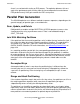
Join With Hash Repartitioning
If both tables are partitioned in a way that does not facilitate parallel execution for
the query, the optimizer can request the executor to repartition (reorganize) both
tables at run time. The matching partitions join algorithm is used on the
reorganized tables.
How the Optimizer Avoids Repartitioning for a Join
Repartitioning involves a lot of extra data movement, so the optimizer tries to avoid it
by using a more efficient alternative strategy known as logical partitioning. The
optimizer might choose one of these forms:
•
Logical partition grouping
Logical partition grouping provides the ability to have fewer ESPs than partitions
without repartitioning. The number of ESPs in SQL/MX is determined more by the
number of available CPUs than it is by the number of partitions in the tables. If a
table has more partitions than available CPUs, the optimizer can group the
partitions so that each ESP processes multiple partitions as if they were a single
partition. Each ESP will group adjacent partitions.
For logical partition grouping in hash partitioned tables, a hash partitioned table
can be grouped to have fewer logical partitions, but it can be matched only with
another table that has the same number of original partitions. For example, a table
with 15 partitions can be grouped to have 4 logical partitions. Three of the logical
partitions would have 4 partitions, and one logical partition would have 3 partitions.
However, this table can be matched only with another table with 15 partitions and 4
logical partitions. It cannot be matched with a hash partitioned table with 16
partitions and 4 logical partitions.
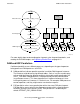
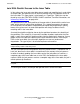
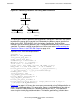
The next figure illustrates logical partition grouping (range partition). The left child
of the join contains two partitions; the right child contains four partitions. Notice,
however, that the partitioning key boundary values of the left child match a subset
of the partitioning key boundary values of the right child. (The left child has a
partitioning key boundary value of 100, and the right child has partitioning key
boundary values of 50, 100, and 150.) The left child is a grouping of the right child,
and the right child is a refinement of the left child. In such circumstances, an ESP
can combine contiguous physical partitions into a single logical partition.
This figure shows how physical partitions 1 and 2 of the right child combine to form
logical partition 1, and how physical partitions 3 and 4 of the right child combine to
form logical partition 2. The logical partitions of the right child match the left child’s
partitioning scheme.