HP NonStop SQL/MX Data Mining Guide Abstract This manual presents a nine-step knowledge-discovery process, which was developed over a series of data mining investigations. This manual describes the data structures and operations of the NonStop™ SQL/MX approach and implementation. Product Version NonStop SQL/MX Release 2.0 Supported Release Version Updates (RVUs) This publication supports G06.23 and all subsequent G-series releases until otherwise indicated by its replacement publication.
Document History Part Number Product Version Published 424397-001 NonStop SQL/MX Release 1.0 February 2001 523737-001 NonStop SQL/MX Release 2.
HP NonStop SQL/MX Data Mining Guide Index Figures What’s New in This Manual iii Manual Information iii New and Changed Information Tables iii About This Manual v Audience v Organization v Related Documentation vi Notation Conventions viii 1.
2. Preparing the Data (continued) Contents 2. Preparing the Data (continued) Moving Metrics 2-9 Rankings 2-10 3. Creating the Data Mining View Creating the Single Table Pivoting the Data 3-3 3-2 4. Mining the Data Building the Model 4-2 Building Decision Trees 4-2 Checking the Model 4-9 Applying the Model to the Mining Table 4-10 Applying the Model to the Database 4-10 Deploying the Model 4-10 Monitoring Model Performance 4-11 A. Creating the Data Mining Database B.
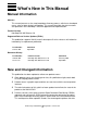
What’s New in This Manual Manual Information HP NonStop SQL/MX Data Mining Guide Abstract This manual presents a nine-step knowledge-discovery process, which was developed over a series of data mining investigations. This manual describes the data structures and operations of the NonStop™ SQL/MX approach and implementation. Product Version NonStop SQL/MX Release 2.0 Supported Release Version Updates (RVUs) This publication supports G06.
New and Changed Information What’s New in This Manual preparation steps in SQL/MX but reserve the mining or model building for UNIX or Microsoft Windows platforms. • • • • • All sections of the manual have been updated to reflect the impact of major changes of SQL/MX Release 2.0 (for example, the introduction of SQL/MX tables). Introductions to the data preparation steps have been revised and rewritten. The DDL statements in Appendix A, B, and C have been updated to use SQL/MX DDL syntax.
About This Manual This manual presents a nine-step knowledge discovery process, which was developed over a series of data mining investigations. This manual describes the data structures and operations of the NonStop SQL/MX approach and implementation. Audience This manual is intended for database administrators and application programmers who are using NonStop SQL/MX to solve data mining problems, either through the SQL conversational interface or through embedded SQL programs.
Related Documentation About This Manual Related Documentation This manual is part of the SQL/MX library of manuals, which includes: Introductory Guides SQL/MX Comparison Guide for SQL/MP Users Describes SQL differences between SQL/MP and SQL/MX. SQL/MX Quick Start Describes basic techniques for using SQL in the SQL/MX conversational interface (MXCI). Includes information about installing the sample database.
Related Documentation About This Manual Specialized Guides SQL/MX Installation and Management Guide Describes how to plan, install, create, and manage an SQL/MX database. Explains how to use installation and management commands and utilities. SQL/MX Query Guide Describes how to understand query execution plans and write optimal queries for an SQL/MX database. SQL/MX Data Mining Guide Describes the SQL/MX data structures and operations to carry out the knowledge-discovery process.
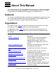
Notation Conventions About This Manual This figure shows the manuals in the SQL/MX library: Programming Manuals Introductory Guides SQL/MX Comparison Guide for SQL/MP Users SQL/MX Programming Manual for C and COBOL SQL/MX Quick Start SQL/MX Programming Manual for Java SQL/MX Guide to Stored Procedures in Java Reference Manuals SQL/MX Reference Manual SQL/MX Messages Manual SQL/MX Glossary SQL/MX Queuing and Publish/ Subscribe Services SQL/MX Query Guide SQL/MX Report Writer Guide DataLoader/
General Syntax Notation About This Manual This requirement is described under Backup DAM Volumes and Physical Disk Drives on page 3-2. General Syntax Notation This list summarizes the notation conventions for syntax presentation in this manual. UPPERCASE LETTERS. Uppercase letters indicate keywords and reserved words. Type these items exactly as shown. Items not enclosed in brackets are required. For example: MAXATTACH lowercase italic letters.
General Syntax Notation About This Manual braces on each side of the list, or horizontally, enclosed in a pair of braces and separated by vertical lines. For example: LISTOPENS PROCESS { $appl-mgr-name } { $process-name } ALLOWSU { ON | OFF } | Vertical Line. A vertical line separates alternatives in a horizontal list that is enclosed in brackets or braces. For example: INSPECT { OFF | ON | SAVEABEND } … Ellipsis.
Notation for Messages About This Manual !i and !o. In procedure calls, the !i notation follows an input parameter (one that passes data to the called procedure); the !o notation follows an output parameter (one that returns data to the calling program). For example: CALL CHECKRESIZESEGMENT ( segment-id , error ) ; !i !o !i,o. In procedure calls, the !i,o notation follows an input/output parameter (one that both passes data to the called procedure and returns data to the calling program).
Notation for Management Programming Interfaces About This Manual [ ] Brackets. Brackets enclose items that are sometimes, but not always, displayed. For example: Event number = number [ Subject = first-subject-value ] A group of items enclosed in brackets is a list of all possible items that can be displayed, of which one or none might actually be displayed.
Notation for Management Programming Interfaces About This Manual lowercase letters. Words in lowercase letters are words that are part of the notation, including Data Definition Language (DDL) keywords. For example: token-type !r. The !r notation following a token or field name indicates that the token or field is required. For example: ZCOM-TKN-OBJNAME !o. token-type ZSPI-TYP-STRING. !r The !o notation following a token or field name indicates that the token or field is optional.
About This Manual Notation for Management Programming Interfaces HP NonStop SQL/MX Data Mining Guide—523737-001 xiv
1 Introduction Knowledge discovery is an iterative process involving many query-intensive steps. The challenges of data management in supporting this process efficiently are significant and continue to grow as knowledge discovery becomes more widely used. Data mining identifies and characterizes interrelationships among multiple variables without requiring a data analyst to formulate specific questions. Software tools look for trends and patterns and flag unusual or potentially interesting ones.
The SQL/MX Approach Introduction algorithms that load the entire data set into memory and perform necessary computations. The extract approach has two major limitations: • • It does not scale to large data sets because the entire data set is required to fit in memory. Statistical sampling can be used to avoid this limitation. However, sampling is inappropriate in many situations because sampling might cause patterns to be missed, such as those in small groups or those between records.
The Knowledge Discovery Process Introduction Building these data structures and operations into the DBMS allows mining tasks to be moved into the SQL engine for tighter integration of data and mining operations and for improved performance and scalability. Adding new primitives, such as moving-window aggregate functions, simplifies queries needed by knowledge discovery tools and applications. This type of query simplification often results in significant improvements in performance.
Defining the Business Opportunity Introduction 6. Create the data mining view. Transform the data into a mining view, a form in which all attributes about the primary mining entity occur in a single record. See Creating the Mining View on page 1-10. 7. Mine the data and build models. Core knowledge discovery techniques are applied to gain insight, learn patterns, or verify hypotheses. The main tasks are either predictive or descriptive in nature.
Defining the Business Opportunity Introduction • Usability of the results Merely identifying patterns is not enough. The opportunity and analysis must be structured so that any interpretation of results obtained develops into deployable business strategy. • Political and organizational reaction In assessing probabilities for organizational resistance, it is helpful to examine similar past efforts and understand why these efforts succeeded or failed.
Defining the Business Opportunity Introduction refined later in the knowledge discovery process as more information becomes available. This manual uses this opportunity scenario to describe the knowledge discovery process and how to implement it. The data set used to illustrate techniques and SQL/MX features consists of two tables: one containing customer information and the other containing account history information. This data set is presented in Appendix A through C of this manual.
Preparing the Data Introduction then a customer is defined as having left—that is, no longer holds a credit card account. Preparing the Data After a business opportunity has been identified and defined, the next task is to prepare a data set for mining. This is done in Steps 2 through 6 of the knowledge discovery process. See The Knowledge Discovery Process on page 1-3. The first two steps are preprocessing the mining data to make it consistent and then loading the data into a database system.
Preparing the Data Introduction You obtain the cardinality of an attribute, which is the count of the number of unique values for the attribute, by using a COUNT DISTINCT query. For example: SELECT COUNT(DISTINCT Age) FROM Customers; or SELECT COUNT(DISTINCT Number_Children) FROM Customers; Instead of having to submit a query for each attribute, you can obtain counts for multiple attributes of a table by using the TRANSPOSE clause. For example: SET NAMETYPE ANSI; SET SCHEMA dmcat.
Preparing the Data Introduction three months before a customer leaves, because these attributes are predictors of attrition. For the customers that do leave, the months leading up to leaving occur at various points in time. For customers that do not leave, these months are chosen to be any three consecutive months in which the account is open. The information about these months should be aligned for all accounts in a single set of columns, one for each of the three months.
Creating the Mining View Introduction Creating the Mining View The final data preparation step is to transform the data set into a mining view, a form in which all attributes about the main mining entity appear in a single record. The mining entity used in this manual is a credit card account. The data mining challenge is to determine predictors for when a customer will close a credit card account.
Knowledge Deployment and Monitoring Introduction Descriptive tasks involve finding patterns describing the data. The most common are: • • • • Database segmentation (clustering)—Map a case into one of several clusters. Summarization—Provide a compact description of the data, often in visual form. Link analysis—Determine relationships between attributes in a case. Sequence analysis—Determine trends over time.
Introduction Knowledge Deployment and Monitoring HP NonStop SQL/MX Data Mining Guide—523737-001 1- 12
2 Preparing the Data Section 1, Introduction identifies and defines a business opportunity, the first step in the knowledge discovery process supported by SQL/MX. This section describes Steps 2 through 5. 1. Identify and define a business opportunity. 2. Preprocess and load the data for the business opportunity. The first preparation step is to address these problems by preprocessing the data in various ways—for example, verifying and mapping the data. Then load the data into your database system.
Loading the Data Preparing the Data Loading the Data The first step in preparing a data set for mining is loading the data into database tables. Suppose the credit card organization has a customers data warehouse. The customer data and the account history data are stored in this warehouse. In a typical real-world scenario, the warehouse could have millions of records representing millions of customers dating back many years.
Cardinalities and Metrics Preparing the Data Cardinalities and Metrics For any attribute, one approach to profiling is to run a separate query for each attribute. As an example, consider the following queries, which profile the discrete attribute Marital Status from the Customers table and the continuous attribute Balance from the Account History table.
Transposition Preparing the Data SELECT attr, c1, COUNT(*) FROM customers TRANSPOSE ('GENDER', gender), ('HOME', home), ('MARITAL_STATUS', marital_status) AS (attr, c1) GROUP BY attr, c1 ORDER BY attr, c1; ATTR -------------GENDER GENDER HOME HOME MARITAL_STATUS MARITAL_STATUS MARITAL_STATUS MARITAL_STATUS C1 -------F M Own Rent Divorced Married Single Widow (EXPR) -------------------20 22 33 9 12 9 15 6 --- 8 row(s) selected.
Quick Profiling Preparing the Data NUMBER_CHILDREN NUMBER_CHILDREN ? ? 2 3 10 3 --- 12 row(s) selected. Because this query produces counts for four different attributes, use the ATTR column to distinguish from which attribute the values are drawn. The C1 column contains the values for the character attributes, and the C2 column contains the values for the numeric attribute.
Defining Events Preparing the Data • • • Randomly sample source data Improve computing efficiency for a profile using a selected sampling percentage Reduce both the I/O costs and the CPU costs associated with computing a profile See the SAMPLE Clause of SELECT in the SQL/MX Reference Manual. Defining Events Events are used to align related data in a single set of columns for mining.
Aligning the Data Preparing the Data is crucial for building models to predict events that occur at different times for each customer. Example of Aligning Data This statement creates an SQL/MX table named Close_Temp that contains the account number, the month the account is considered closed (if not closed, an arbitrary month), and an indicator of whether or not the customer left: SET SCHEMA mining.
Aligning the Data Preparing the Data THEN m.year_month END FROM acct_history m SEQUENCE BY m.account, m.year_month) t (account, year_month, close_month1, close_month2) GROUP BY t.account) p (account, close_month1, close_month2, open_month)); The derived attribute Close_Month1 contains the month when a customer explicitly closed their account (the Account Status is marked Closed).
Deriving Attributes Preparing the Data Account Number Close Month Cust_Left 4300000 1999-06-01 N 4400000 1999-07-01 Y 4500000 1998-09-01 Y 4600000 1999-12-01 Y 4700000 1999-06-01 N Deriving Attributes In the preceding Example of Aligning Data on page 2-7, the derived attributes in the Close_Temp table are Close_Month and Cust_Left.
Rankings Preparing the Data 1000000 1000000 ... 1998-12-01 1999-01-01 ... 5134.22 4572.19 ... --- 186 row(s) selected. In this query, the ROWS SINCE INCLUSIVE sequence function is used to limit the moving average window to records for the current customer. The third argument of MOVINGAVG is RUNNINGCOUNT(*), which ensures MOVINGAVG does not include rows before the beginning row.
3 Creating the Data Mining View Because data mining often involves executing a series of similar queries before getting satisfying results, it can be helpful to use materialized results of previous queries when answering a new one. Creating a data mining view allows you to access intentionally gathered and permanently stored results of a data mining query. Creating a data mining view is Step 6 of the knowledge discovery process. 1. Identify and define a business opportunity. 2.
Creating the Data Mining View Creating the Single Table Creating the Single Table After computing derived attributes and storing these attributes in auxiliary tables, you create the mining view by combining all the information into a single table with one row for each entity. Continuing with the credit card example, the mining view contains the information in the Customers table along with the auxiliary customer data. In addition, information in the Account History and related tables is also used.
Creating the Data Mining View Pivoting the Data NOT NULL NUMERIC (9,2) NO DEFAULT NOT NULL ,cust_left CHAR(1) NO DEFAULT ,PRIMARY KEY (account) ); ,balance_close_3 Pivoting the Data All the data in the Customer, Account History, and auxiliary tables must be collapsed to a single row for each customer. Collapsing the data is accomplished by pivoting the data. Data is purged from separate rows for each customer into different columns of a single customer row.
Pivoting the Data Creating the Data Mining View END AS balance_close_3 ,cust_left FROM acct_history a NATURAL JOIN close_temp m SEQUENCE BY account, year_month) AS t, customers c WHERE t.balance_close_1 IS NOT NULL AND t.balance_close_2 IS NOT NULL AND t.balance_close_3 IS NOT NULL AND c.account = t.account); Sequence functions are used in the preceding query to create a derived table with the various balances for each customer.
Pivoting the Data Creating the Data Mining View Account Number ... Year_ Month Close Month Balance Close_1 Balance Close_2 Balance Close_3 3900000 1998-10-01 4098124 1998-10-01 .00 .00 .00 Y 1998-10-01 1998-10-01 4069.34 4347.63 4596.10 Y 4300000 1999-06-01 1999-06-01 9000.00 4354.00 9876.00 N 4400000 1999-07-01 1999-07-01 .00 .00 .00 Y 4500000 1998-09-01 1998-09-01 .00 100.00 50.00 Y 4600000 1999-12-01 1999-12-01 1000.00 50.00 80.
Creating the Data Mining View HP NonStop SQL/MX Data Mining Guide—523737-001 3 -6 Pivoting the Data
4 Mining the Data This section describes the next three steps of the process, Steps 7 through 9. 1. Identify and define a business opportunity. 2. Preprocess and load the data for the business opportunity. 3. Profile and understand the relevant data. 4. Define events relevant to the business opportunity being explored. 5. Derive attributes. 6. Create the data mining view. 7. Mine the data and build models.
Building the Model Mining the Data Building the Model Typically, after the mining view is computed and inserted into a single database table, the data is extracted and loaded into a mining tool for the model building step. Regardless of the type of analysis to be performed, the mining data can be stored and retrieved by using the SQL/MX approach. This subsection describes how a decision tree can be used for data analysis.
Building Decision Trees Mining the Data GENDER MARITAL STATUS MARITAL STATUS MARITAL STATUS MARITAL STATUS MARITAL STATUS MARITAL STATUS MARITAL STATUS NUMBER_CHILDREN NUMBER_CHILDREN NUMBER_CHILDREN NUMBER_CHILDREN NUMBER_CHILDREN NUMBER_CHILDREN M Divorced Divorced Married Married Single Widow Widow ? ? ? ? ? ? ? ? ? ? ? ? ? ? 0 0 1 2 2 3 Y N Y N Y Y N Y N Y Y N Y N 6 1 5 2 1 3 1 1 2 5 2 1 3 1 --- 17 row(s) selected.
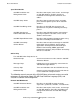
Building Decision Trees Mining the Data Typically, the best discriminator of the goal is determined by a statistical analysis of the cross tables. The exact nature of this analysis varies from tool to tool. Initial Decision Tree Figure 4-1 shows the initial decision tree for the business opportunity. Marital Status is chosen as the best predictor of the goal with four initial branches—Divorced, Single, Married, and Widow. Figure 4-1.
Building Decision Trees Mining the Data GENDER NUMBER_CHILDREN NUMBER_CHILDREN NUMBER_CHILDREN NUMBER_CHILDREN M ? 0 0 1 2 ? ? ? ? Y N Y Y Y 5 1 1 1 3 --- 6 row(s) selected. The preceding query shows Gender is Male in all cases where Cust_Left is equal to Y, and therefore Gender is a good predictor where Marital Status is Divorced. The Number_Children is equal to 0, 1, and 2, and therefore Number_Children is not a good predictor.
Building Decision Trees Mining the Data -------------------GENDER GENDER NUMBER_CHILDREN --F M ? -----? ? 0 --------Y Y Y -------2 1 3 --- 3 row(s) selected. The preceding query shows split results for Gender when Cust_Left is equal to Y, and therefore Gender is not a good predictor when Marital Status equal to Single. However, the query also shows Number_Children equal to 0 when Cust_Left is equal to Y, and therefore Number_Children is a good predictor.
Building Decision Trees Mining the Data Showing the Homogeneous Branches For each of the preceding conditions, these queries show that he branches in the decision tree are homogeneous with respect to the goal attribute Cust_Left.
Building Decision Trees Mining the Data Computing Cross Table When Marital Status is Single and Children is Zero This query generates cross tables for the Number_Children attribute compared to the goal when Marital Status is Single and Number_Children is 0: SELECT Independent_Variable, IV2, cust_left, COUNT(*) FROM miningview WHERE marital_status = 'Single' AND number_children = 0 TRANSPOSE ('NUMBER_CHILDREN', number_children) AS (Independent_Variable, IV2) GROUP BY Independent_Variable, IV2, cust_left OR
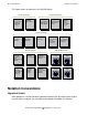
Checking the Model Mining the Data Figure 4-4 shows the final decision tree for the example business opportunity. Figure 4-4. Final Decision Tree Marital Status Divorced No Yes 1 5 Male No Yes 0 5 Single No Yes 0 3 Female No Yes 1 0 Chldrn=0 No Yes 0 3 Chldrn>0 No Yes 0 0 Married No Yes 2 1 Widow No Yes 1 1 Prune the tree here because the remaining branches do not yield a pattern.
Applying the Model to the Mining Table Mining the Data Applying the Model to the Mining Table You must check your model against the mining table.
Monitoring Model Performance Mining the Data Monitoring Model Performance When measuring a model, consider these questions: • How accurate is the model? The accuracy of the model can be measured as a whole. For example, you can determine the percentage of records that are classified correctly. The accuracy of the parts of a model can also be measured. For example, in a decision tree, each branch of the tree has an associated error rate.
Mining the Data Monitoring Model Performance HP NonStop SQL/MX Data Mining Guide—523737-001 4- 12
A Creating the Data Mining Database The examples presented in this manual use tables created by the execution of SQL/MX CREATE TABLE statements. These SQL/MX DDL statements enable you to create the data mining database so that you can use the SQL/MX features shown in this manual.
Creating the Data Mining Database ,age NUMERIC (3) DEFAULT NULL HEADING 'Age' ,number_children NUMERIC (2) DEFAULT null HEADING 'Number of Children' ,PRIMARY KEY (account) NOT DROPPABLE ) LOCATION $P2 PARTITION (ADD FIRST KEY 3000000 LOCATION $VOLUME, ADD FIRST KEY 5000000 LOCATION $P1); -- Set constraint on home column; must be Rent or Own or NULL ALTER TABLE customers ADD CONSTRAINT home_constraint CHECK (home = 'Own' OR home = 'Rent' OR home IS NULL); -- Set constraint on marital status column; must be
Creating the Data Mining Database NO DEFAULT NOT NULL NOT DROPPABLE ,status CHAR (10) NO DEFAULT NOT NULL NOT DROPPABLE ,cust_limit NUMERIC (9,2) NO DEFAULT NOT NULL NOT DROPPABLE ,balance NUMERIC (9,2) NO DEFAULT NOT NULL NOT DROPPABLE ,payment NUMERIC (9,2) NO DEFAULT NOT NULL NOT DROPPABLE ,finance_charge NUMERIC (9,2) NO DEFAULT NOT NULL NOT DROPPABLE ,PRIMARY KEY (account, year_month) ) LOCATION $P2 PARTITION (ADD FIRST KEY 3000000 LOCATION $VOLUME, ADD FIRST KEY 5000000 LOCATION $P1); -- Set constra
Creating the Data Mining Database HP NonStop SQL/MX Data Mining Guide—523737-001 A- 4
B Inserting Into the Data Mining Database The following INSERT statements enable you to populate the data mining database. Use the following script to populate the CUSTOMERS table and the ACCT_HISTORY table: -------------------------------------------------------------- Data mining database in catalog dmcat and schema whse -- Run this script in MXCI -------------------------------------------------------------- POPULATE THE DATA MINING DATABASE TABLES SET SCHEMA dmcat.
Inserting Into the Data Mining Database (7900000,'LAUREN','LITTLE', 'Widow', 'Own', 28000,'F',65,0), (8000000,'BRENT', 'BLACK', 'Married', 'Own', 175500,'M',45,3), (8100000,'STEVEN','HUFF', 'Widow', 'Own', 137000,'M',42,2), (8200000,'ELLIE', 'RAYMOND','Married', 'Rent',136000,'F',50,0), (8300000,'PATRICK','ZORO', 'Divorced','Rent',138000,'M',40,1), (8400000,'SHAWN', 'JONES', 'Divorced','Own', 75000,'M',40,2), (8500000,'ABBIE', 'LAUREN', 'Single', 'Own', 200000,'F',19,0), (8600000,'ELSIE', 'VANDER', 'Single
Inserting Into the Data Mining Database (2500000,DATE (2500000,DATE (2500000,DATE (2500000,DATE (2500000,DATE '2003-08-01','Open', '2003-09-01','Open', '2003-10-01','Open', '2003-11-01','Open', '2003-12-01','Open', 5000, 5000, 5000, 5000, 5000, 0, 0, 0, 0, 0, 0, 0, 0, 0, 0, 0), 0), 0), 0), 0); INSERT INTO acct_history VALUES (4098124,DATE '2000-10-01','Open', 6000,32000.00,3200.00,0.00), (4098124,DATE '2000-11-01','Open', 6000, 2300.00,2300.00,0.00), (4098124,DATE '2000-12-01','Open', 6000, 0.00, 0.
Inserting Into the Data Mining Database INSERT INTO acct_history VALUES (1000000,DATE '2002-07-01','Open',20000,3678.67,3678.67, 0.00), (1000000,DATE '2002-08-01','Open',20000,6780.00,6780.00, 0.00), (1000000,DATE '2002-09-01','Open',20000,2300.78,2300.78, 0.00), (1000000,DATE '2002-10-01','Open',20000,8000.00,8000.00, 0.00), (1000000,DATE '2002-11-01','Open',20000,5345.89,5345.89, 0.00), (1000000,DATE '2002-12-01','Open',20000,4700.00,4700.00, 0.00), (1000000,DATE '2003-01-01','Open',20000,1200.00,1200.
Inserting Into the Data Mining Database (2900000,DATE '2003-11-01','Open',15000, 2000.00, 2000.00, 0), (2900000,DATE '2003-12-01','Open',15000, 5890.00, 5890.
Inserting Into the Data Mining Database (4400000,DATE (4400000,DATE (4400000,DATE (4400000,DATE (4400000,DATE (4400000,DATE (4400000,DATE (4400000,DATE (4400000,DATE (4400000,DATE (4400000,DATE '2003-02-01','Open',40000, '2003-03-01','Open',40000, '2003-04-01','Open',40000, '2003-05-01','Open',40000, '2003-06-01','Open',40000, '2003-07-01','Open',40000, '2003-08-01','Open',40000, '2003-09-01','Open',40000, '2003-10-01','Open',40000, '2003-11-01','Open',40000, '2003-12-01','Open',40000, 100.00, 50.00, 90.
C Importing Into the Data Mining Database The format file, data file, and the import command provided in this appendix enable you to populate the data mining database. You cannot execute the import utility command through MXCI or in programs. You must run import at the command prompt. For further information, see the import Utility entry in the NonStop SQL/MX Reference Manual. Importing Customers Data The import command for the Customers table looks like this: IMPORT dmcat.whse.customers -I importdatac.
Importing Into the Data Mining Database Importing Account History Data 1000000,ROGER,GREEN,Married,Own,175500,M,45,3 2300000,JERRY,HOWARD,Divorced,Own,137000,M,42,2 2900000,JANE,RAYMOND,Divorced,Rent,136000,F,50,0 3200000,THOMAS,RUDLOFF,Divorced,Rent,138000,M,40,1 3900000,KLAUS,SAFFERT,Divorced,Own,75000,M,40,2 4300000,DEBBIE,DUNN,Married,Own,300000,F,29,2 4400000,HANNAH,ROSE,Single,Own,300000,F,29,0 4500000,LIZ,STONE,Married,Own,300000,F,29,1 4600000,HANS,NOBLE,Single,Own,300000,M,48,0 4700000,SEAN,FREDR
Importing Into the Data Mining Database Account History Format File Account History Format File This file is named importfmta.txt and is the format file specified in the preceding import command: [DATE FORMAT] DateOrder=YMD DateDelimiter=[COLUMN FORMAT] col=account,N col=year_month,N col=status,N col=cust_limit,N col=balance,N col=payment,N col=finance_charge,N [DELIMITED FORMAT] FieldDelimiter=, Account History Data File This file is named importdataa.
Importing Into the Data Mining Database Account History Data File 2500000,2003-07-01,Open,5000,834.40,834.40,0 2500000,2003-08-01,Open,5000,0,0,0 2500000,2003-09-01,Open,5000,0,0,0 2500000,2003-10-01,Open,5000,0,0,0 2500000,2003-11-01,Open,5000,0,0,0 2500000,2003-12-01,Open,5000,0,0,0 4098124,2000-10-01,Open,6000,32000.00,3200.00,0.00 4098124,2000-11-01,Open,6000,2300.00,2300.00,0.00 4098124,2000-12-01,Open,6000,0.00,0.00,0.00 4098124,2001-01-01,Open,6000,0.00,0.00,0.00 4098124,2001-02-01,Open,6000,4000.
Importing Into the Data Mining Database Account History Data File 1000000,2002-11-01,Open,20000,5345.89,5345.89,0.00 1000000,2002-12-01,Open,20000,4700.00,4700.00,0.00 1000000,2003-01-01,Open,20000,1200.00,1200.00,0.00 1000000,2003-02-01,Delinquent,20000,3500.00,0.00,51.75 1000000,2003-03-01,Open,20000,5500.00,5500.00,0.00 1000000,2003-04-01,Open,20000,0.00,0.00,0.00 1000000,2003-05-01,Open,20000,6500.00,6500.00,0.00 1000000,2003-06-01,Open,20000,4590.00,4590.00,0.00 1000000,2003-07-01,Open,20000,3200.
Importing Into the Data Mining Database Account History Data File 3200000,2003-02-01,Open,10000,800.00,800.00,0 3200000,2003-03-01,Open,10000,0,0,0 3200000,2003-04-01,Open,10000,0,0,0 3200000,2003-05-01,Open,10000,0,0,0 3200000,2003-06-01,Open,10000,0,0,0 3900000,20012000-12-01,Open,5000,800.00,800.00,0 3900000,2002-01-01,Open,5000,300.00,300.00,0 3900000,2002-02-01,Open,5000,230.00,230.00,0 3900000,2002-03-01,Open,5000,789.00,789.00,0 3900000,2002-04-01,Open,5000,600.00,600.
Importing Into the Data Mining Database Account History Data File 4600000,2003-04-01,Open,40000,30.00,30.00,0 4600000,2003-05-01,Open,40000,30.00,30.00,0 4600000,2003-06-01,Open,40000,30.00,30.00,0 4600000,2003-07-01,Open,40000,30.00,30.00,0 4600000,2003-08-01,Open,40000,60.00,60.00,0 4600000,2003-09-01,Open,40000,700.00,700.00,0 4600000,2003-10-01,Open,40000,80.00,80.00,0 4600000,2003-11-01,Open,40000,50.00,50.00,0 4600000,2003-12-01,Closed,40000,1000.00,1000.00,0 4700000,2003-01-01,Open,40000,330.
Importing Into the Data Mining Database HP NonStop SQL/MX Data Mining Guide—523737-001 C- 8 Account History Data File
Index A Aligning data 1-9, 2-6 Attributes cardinality of 1-7, 2-3 continuous 2-3, 2-5 deriving 2-9 discrete 1-7, 2-3 discrete numeric 2-4 statistics 2-5 Decision trees cross tables 4-2 dependent variable 4-2 description of 4-2 first branch 4-2 goal definition 4-6 goal prediction 4-3 independent variables 4-2 Defining events 1-8, 2-6 Deploying model 1-11, 4-10 B K Business model building 4-2 checking against database 4-9 deploying 4-10 monitoring 4-11 summarizing results 4-8 Business opportunity defining
R Index R Rankings 2-10 ROWS SINCE function 2-7, 2-9 RUNNINGCOUNT function 2-10 S SEQUENCE BY clause 2-8, 2-9, 2-10, 3-4 SQL/MX approach, advantages of 1-2 T THIS function 2-9 TRANSPOSE clause 2-4, 2-5, 4-2, 4-4 1-8 Transposition 2-3 V VARIANCE set function 2-3, 2-5 HP NonStop SQL/MX Data Mining Guide—523737-001 Index -2