
Service manual


8.0 APPLICATIONS
8.1 General
XR Series power supplies deploy several powerful programming functions that enhance
performance for user specific applications. While the possibilities are endless, a few examples
are presented in this chapter to demonstrate the internal capabilities of the power supply. All of
these examples can be further expanded by operating the unit under computer control.
8.2 Leadless Remote Sensing
Remote sensing is used to improve the degradation of regulation which will occur at the load
when the voltage drop in the connecting wires is appreciable. Remote sensing, as described in
Section 3.3, requires an pair of wires to be connected between the output of the power supply and
the desired point of load regulation. Remote sensing can be accomplished, without the use of the
additional sense leads, by calculating the voltage drop in the output leads and adjusting the output
voltage accordingly.
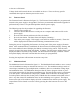
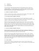
To establish leadless remote sensing, connect terminal 24 of JS1 to terminal 25 of JS1, set the
modulation control parameter to voltage control, and set the modulation type to 1. Figure 8.1
illustrates the hardware connection and Section 4.3.14 describes application of the modulation
subsystem. With this configuration, output voltage will increase or decrease with output current
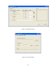
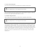
as defined by the modulation table. By programming a positive slope into the modulation table,
output voltage and voltage drop due to lead loss can be made to cancel. For an installation where
there is a 2% drop in voltage at full scale current, the modulation table should be programmed
according to Table 8.1. For row 3 in the modulation table, VMOD is given the value 9999 to
signify the last entry.
8.3 Photovoltaic Cell Simulator
Modulation enables the power supply to emulate different sources: such as batteries, fuel cells,
photovoltaic arrays, etc. To simulate a photovoltaic array, connect terminal 24 of JS1 to terminal
25 of JS1, set the modulation control parameter to voltage control, and set the modulation type to
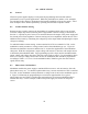
0. Figure 8.2 illustrates the programmed piece-wise linear approximation for a typical
photovoltaic array and Table 8.2 defines the associated piece-wise linear modulation table to
emulate that array. For this example, a XR125-48 power supply was chosen for the power
source.
98