
Specifications
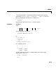
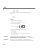
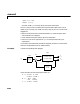
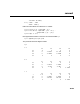
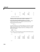
Table Of Contents
- Introduction
- LTI Models
- Operations on LTI Models
- Model Analysis Tools
- Arrays of LTI Models
- Customization
- Setting Toolbox Preferences
- Setting Tool Preferences
- Customizing Response Plot Properties
- Design Case Studies
- Reliable Computations
- GUI Reference
- SISO Design Tool Reference
- Menu Bar
- File
- Import
- Export
- Toolbox Preferences
- Print to Figure
- Close
- Edit
- Undo and Redo
- Root Locus and Bode Diagrams
- SISO Tool Preferences
- View
- Root Locus and Bode Diagrams
- System Data
- Closed Loop Poles
- Design History
- Tools
- Loop Responses
- Continuous/Discrete Conversions
- Draw a Simulink Diagram
- Compensator
- Format
- Edit
- Store
- Retrieve
- Clear
- Window
- Help
- Tool Bar
- Current Compensator
- Feedback Structure
- Root Locus Right-Click Menus
- Bode Diagram Right-Click Menus
- Status Panel
- Menu Bar
- LTI Viewer Reference
- Right-Click Menus for Response Plots
- Function Reference
- Functions by Category
- acker
- allmargin
- append
- augstate
- balreal
- bode
- bodemag
- c2d
- canon
- care
- chgunits
- connect
- covar
- ctrb
- ctrbf
- d2c
- d2d
- damp
- dare
- dcgain
- delay2z
- dlqr
- dlyap
- drss
- dsort
- dss
- dssdata
- esort
- estim
- evalfr
- feedback
- filt
- frd
- frdata
- freqresp
- gensig
- get
- gram
- hasdelay
- impulse
- initial
- interp
- inv
- isct, isdt
- isempty
- isproper
- issiso
- kalman
- kalmd
- lft
- lqgreg
- lqr
- lqrd
- lqry
- lsim
- ltimodels
- ltiprops
- ltiview
- lyap
- margin
- minreal
- modred
- ndims
- ngrid
- nichols
- norm
- nyquist
- obsv
- obsvf
- ord2
- pade
- parallel
- place
- pole
- pzmap
- reg
- reshape
- rlocus
- rss
- series
- set
- sgrid
- sigma
- sisotool
- size
- sminreal
- ss
- ss2ss
- ssbal
- ssdata
- stack
- step
- tf
- tfdata
- totaldelay
- zero
- zgrid
- zpk
- zpkdata
- Index

connect
16-39
-13.5009 18.0745];
D = [-.5476 -.1410
-.6459 .2958 ];
Define the three blocks as individual LTI models.
sys1 = tf(10,[1 5],'inputname','uc')
sys2 = ss(A,B,C,D,'inputname',{'u1' 'u2'},...
'outputname',{'y1' 'y2'})
sys3 = zpk(-1,-2,2)
Next append these blocks to form the unconnected model sys.
sys = append(sys1,sys2,sys3)
This produces the block-diagonal model
sys
a =
x1 x2 x3 x4
x1 -5 0 0 0
x2 0 -9.0201 17.779 0
x3 0 -1.6943 3.2138 0
x4 0 0 0 -2
b =
uc u1 u2 ?
x1 4 0 0 0
x2 0 -0.5112 0.5362 0
x3 0 -0.002 -1.847 0
x4 0 0 0 1.4142
c =
x1 x2 x3 x4
? 2.5 0 0 0
y1 0 -3.2897 2.4544 0
y2 0 -13.501 18.075 0
? 0 0 0 -1.4142