
User`s guide
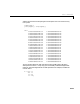
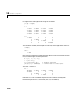
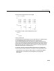
Table Of Contents
- Preface
- Quick Start
- LTI Models
- Introduction
- Creating LTI Models
- LTI Properties
- Model Conversion
- Time Delays
- Simulink Block for LTI Systems
- References
- Operations on LTI Models
- Arrays of LTI Models
- Model Analysis Tools
- The LTI Viewer
- Introduction
- Getting Started Using the LTI Viewer: An Example
- The LTI Viewer Menus
- The Right-Click Menus
- The LTI Viewer Tools Menu
- Simulink LTI Viewer
- Control Design Tools
- The Root Locus Design GUI
- Introduction
- A Servomechanism Example
- Controller Design Using the Root Locus Design GUI
- Additional Root Locus Design GUI Features
- References
- Design Case Studies
- Reliable Computations
- Reference
- Category Tables
- acker
- append
- augstate
- balreal
- bode
- c2d
- canon
- care
- chgunits
- connect
- covar
- ctrb
- ctrbf
- d2c
- d2d
- damp
- dare
- dcgain
- delay2z
- dlqr
- dlyap
- drmodel, drss
- dsort
- dss
- dssdata
- esort
- estim
- evalfr
- feedback
- filt
- frd
- frdata
- freqresp
- gensig
- get
- gram
- hasdelay
- impulse
- initial
- inv
- isct, isdt
- isempty
- isproper
- issiso
- kalman
- kalmd
- lft
- lqgreg
- lqr
- lqrd
- lqry
- lsim
- ltiview
- lyap
- margin
- minreal
- modred
- ndims
- ngrid
- nichols
- norm
- nyquist
- obsv
- obsvf
- ord2
- pade
- parallel
- place
- pole
- pzmap
- reg
- reshape
- rlocfind
- rlocus
- rltool
- rmodel, rss
- series
- set
- sgrid
- sigma
- size
- sminreal
- ss
- ss2ss
- ssbal
- ssdata
- stack
- step
- tf
- tfdata
- totaldelay
- zero
- zgrid
- zpk
- zpkdata
- Index

10 Reliable Computations
10-12
Its eigenvectors and eigenvalues are given as follows.
[v,d] = eig(A)
v =
0.7071 –0.0000 –0.3162 0.6325
–0.7071 0.0000 –0.3162 0.6325
0.0000 0.7071 0.6325 0.3162
–0.0000 –0.7071 0.6325 0.3162
d =
1.0000 0 0 0
0 2.0000 0 0
0 0 5.0000 0
0 0 0 10.0000
The condition number (with respect to inversion) of the eigenvector matrix is
cond(v)
ans =
1.000
Now convert a state-space model with the above A matrix to transfer function
form, and back again to state-sp ace form.
b = [1 ; 1 ; 0 ; –1];
c = [0 0 2 1];
H = tf(ss(A,b,c,0)); % transfer function
[Ac,bc,cc] = ssdata(H) % convert back to state space
The new A matrix is
Ac =
18.0000 –6.0625 2.8125 –1.5625
16.0000 0 0 0
0 4.0000 0 0
0 0 1.0000 0
Note that Ac is not a standard companion matrix and has already been
balanced as part of the
ss conversion (see ssbal for details).