
User`s guide
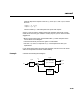
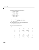

Table Of Contents
- Preface
- Quick Start
- LTI Models
- Introduction
- Creating LTI Models
- LTI Properties
- Model Conversion
- Time Delays
- Simulink Block for LTI Systems
- References
- Operations on LTI Models
- Arrays of LTI Models
- Model Analysis Tools
- The LTI Viewer
- Introduction
- Getting Started Using the LTI Viewer: An Example
- The LTI Viewer Menus
- The Right-Click Menus
- The LTI Viewer Tools Menu
- Simulink LTI Viewer
- Control Design Tools
- The Root Locus Design GUI
- Introduction
- A Servomechanism Example
- Controller Design Using the Root Locus Design GUI
- Additional Root Locus Design GUI Features
- References
- Design Case Studies
- Reliable Computations
- Reference
- Category Tables
- acker
- append
- augstate
- balreal
- bode
- c2d
- canon
- care
- chgunits
- connect
- covar
- ctrb
- ctrbf
- d2c
- d2d
- damp
- dare
- dcgain
- delay2z
- dlqr
- dlyap
- drmodel, drss
- dsort
- dss
- dssdata
- esort
- estim
- evalfr
- feedback
- filt
- frd
- frdata
- freqresp
- gensig
- get
- gram
- hasdelay
- impulse
- initial
- inv
- isct, isdt
- isempty
- isproper
- issiso
- kalman
- kalmd
- lft
- lqgreg
- lqr
- lqrd
- lqry
- lsim
- ltiview
- lyap
- margin
- minreal
- modred
- ndims
- ngrid
- nichols
- norm
- nyquist
- obsv
- obsvf
- ord2
- pade
- parallel
- place
- pole
- pzmap
- reg
- reshape
- rlocfind
- rlocus
- rltool
- rmodel, rss
- series
- set
- sgrid
- sigma
- size
- sminreal
- ss
- ss2ss
- ssbal
- ssdata
- stack
- step
- tf
- tfdata
- totaldelay
- zero
- zgrid
- zpk
- zpkdata
- Index

connect
11-36
Given the matrices of the state-space model sys2
A = [ –9.0201 17.7791
–1.6943 3.2138 ];
B = [ –.5112 .5362
–.002 –1.8470];
C = [ –3.2897 2.4544
–13.5009 18.0745];
D = [–.5476 –.1410
–.6459 .2958 ];
Define the three blocks as individual LTI models.
sys1 = tf(10,[1 5],'inputname','uc')
sys2 = ss(A,B,C,D,'inputname',{'u1' 'u2'},...
'outputname',{'y1' 'y2'})
sys3 = zpk(–1,–2,2)
Next append these blocks to form the unconnected model sys.
sys = append(sys1,sys2,sys3)
This produces the block-diagonal model
sys
a =
x1 x2 x3 x4
x1 -5 0 0 0
x2 0 -9.0201 17.779 0
x3 0 -1.6943 3.2138 0
x4 0 0 0 -2
b =
uc u1 u2 ?
x1 4 0 0 0
x2 0 -0.5112 0.5362 0
x3 0 -0.002 -1.847 0
x4 0 0 0 1.4142