
User`s guide
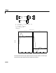
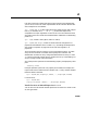
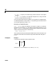
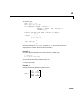
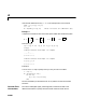
Table Of Contents
- Preface
- Quick Start
- LTI Models
- Introduction
- Creating LTI Models
- LTI Properties
- Model Conversion
- Time Delays
- Simulink Block for LTI Systems
- References
- Operations on LTI Models
- Arrays of LTI Models
- Model Analysis Tools
- The LTI Viewer
- Introduction
- Getting Started Using the LTI Viewer: An Example
- The LTI Viewer Menus
- The Right-Click Menus
- The LTI Viewer Tools Menu
- Simulink LTI Viewer
- Control Design Tools
- The Root Locus Design GUI
- Introduction
- A Servomechanism Example
- Controller Design Using the Root Locus Design GUI
- Additional Root Locus Design GUI Features
- References
- Design Case Studies
- Reliable Computations
- Reference
- Category Tables
- acker
- append
- augstate
- balreal
- bode
- c2d
- canon
- care
- chgunits
- connect
- covar
- ctrb
- ctrbf
- d2c
- d2d
- damp
- dare
- dcgain
- delay2z
- dlqr
- dlyap
- drmodel, drss
- dsort
- dss
- dssdata
- esort
- estim
- evalfr
- feedback
- filt
- frd
- frdata
- freqresp
- gensig
- get
- gram
- hasdelay
- impulse
- initial
- inv
- isct, isdt
- isempty
- isproper
- issiso
- kalman
- kalmd
- lft
- lqgreg
- lqr
- lqrd
- lqry
- lsim
- ltiview
- lyap
- margin
- minreal
- modred
- ndims
- ngrid
- nichols
- norm
- nyquist
- obsv
- obsvf
- ord2
- pade
- parallel
- place
- pole
- pzmap
- reg
- reshape
- rlocfind
- rlocus
- rltool
- rmodel, rss
- series
- set
- sgrid
- sigma
- size
- sminreal
- ss
- ss2ss
- ssbal
- ssdata
- stack
- step
- tf
- tfdata
- totaldelay
- zero
- zgrid
- zpk
- zpkdata
- Index

step
11-221
All systems must have the same number of inputs and outputs b ut may
otherwise be a mix of continuous- and discrete-time systems. This syntax is
useful to compare the step responses of multiple s ystems.
You can also specify a distinctive color, linestyle, and/or marker for each
system. For example,
step(sys1,'y:',sys2,'g--')
plots the step response of sys1 with a dotted yellow line and the step response
of
sys2 with a green dashed line.
When i nvoked with output arguments,
[y,t] = step(sys)
[y,t,x] = step(sys) % for state-space models only
y = step(sys,t)
return the output response y, the time vector t used for simulation, and the
state trajectories
x (for state-space models only). No plot is drawn on the
screen. For single-input systems,
y hasasmanyrowsastimesamples(length
of
t), and as many columns as outputs. In the multi-input ca se, the step
responses of each input channel a re stacked up along the third dimension of
y.
The dimensions of
y are then
and
y(:,:,j) gives the response to a unit step command injected in the jth
input channel. Similarly , the dimensions of
x are
Example Plot the step response of the following second-order state-space model.
length of
t()
number of outputs
()
number of inputs
()××
length of
t()
number of states
()
number of inputs
()××