
User`s guide
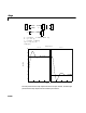
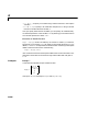
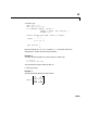
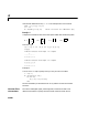
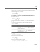
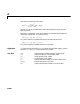
Table Of Contents
- Preface
- Quick Start
- LTI Models
- Introduction
- Creating LTI Models
- LTI Properties
- Model Conversion
- Time Delays
- Simulink Block for LTI Systems
- References
- Operations on LTI Models
- Arrays of LTI Models
- Model Analysis Tools
- The LTI Viewer
- Introduction
- Getting Started Using the LTI Viewer: An Example
- The LTI Viewer Menus
- The Right-Click Menus
- The LTI Viewer Tools Menu
- Simulink LTI Viewer
- Control Design Tools
- The Root Locus Design GUI
- Introduction
- A Servomechanism Example
- Controller Design Using the Root Locus Design GUI
- Additional Root Locus Design GUI Features
- References
- Design Case Studies
- Reliable Computations
- Reference
- Category Tables
- acker
- append
- augstate
- balreal
- bode
- c2d
- canon
- care
- chgunits
- connect
- covar
- ctrb
- ctrbf
- d2c
- d2d
- damp
- dare
- dcgain
- delay2z
- dlqr
- dlyap
- drmodel, drss
- dsort
- dss
- dssdata
- esort
- estim
- evalfr
- feedback
- filt
- frd
- frdata
- freqresp
- gensig
- get
- gram
- hasdelay
- impulse
- initial
- inv
- isct, isdt
- isempty
- isproper
- issiso
- kalman
- kalmd
- lft
- lqgreg
- lqr
- lqrd
- lqry
- lsim
- ltiview
- lyap
- margin
- minreal
- modred
- ndims
- ngrid
- nichols
- norm
- nyquist
- obsv
- obsvf
- ord2
- pade
- parallel
- place
- pole
- pzmap
- reg
- reshape
- rlocfind
- rlocus
- rltool
- rmodel, rss
- series
- set
- sgrid
- sigma
- size
- sminreal
- ss
- ss2ss
- ssbal
- ssdata
- stack
- step
- tf
- tfdata
- totaldelay
- zero
- zgrid
- zpk
- zpkdata
- Index

tf
11-229
engineers use the variable a nd order the numerator and denominator terms
in descending powers of , for example,
The polynomials and are then specified by the row vectors
[1 0 0] and [1 2 3], respectively. By contrast, DSP engineers prefer to write
this trans fer function as
and specify its numerator as
1 (instead of [1 0 0]) and its denominator as
[1 2 3].
tf switches convention based on your choice of variable (value of the
'Variable' property).
For example,
g = tf([1 1],[1 2 3],0.1)
specifies the discrete transfer function
because is the default variable. In contrast,
h = tf([1 1],[1 2 3],0.1,'variable','z^–1')
Variable Convention
'z'
(default) Use the row vector [ak ... a1 a0] to specify the
polynomial (coefficients ordered in
descending powers of ).
'z^–1', 'q' Use the row vector [b0 b1 ... bk] to specify t he
polynomial (coefficients in
ascending powers of or ).
z
z
hz()
z
2
z
2
2z 3++
----------------------------=
z
2
z
2
2 z 3++
hz
1–
()
1
12z
1–
3z
2–
++
----------------------------------------=
a
k
z
k
... a
1
za
0
++ +
z
b
0
b
1
z
1
–
... b
k
z
k
–
+++
z
1
–
q
gz()
z 1
+
z
2
2z 3++
----------------------------=
z