Curve Fitting Toolbox For Use with MATLAB ® Computation Visualization Programming User’s Guide Version 1
How to Contact The MathWorks: www.mathworks.com comp.soft-sys.matlab Web Newsgroup info@mathworks.com Technical support Product enhancement suggestions Bug reports Documentation error reports Order status, license renewals, passcodes Sales, pricing, and general information 508-647-7000 Phone 508-647-7001 Fax The MathWorks, Inc. 3 Apple Hill Drive Natick, MA 01760-2098 Mail support@mathworks.com suggest@mathworks.com bugs@mathworks.com doc@mathworks.com service@mathworks.
Contents Preface What Is the Curve Fitting Toolbox? . . . . . . . . . . . . . . . . . . . . . . vi Exploring the Toolbox . . . . . . . . . . . . . . . . . . . . . . . . . . . . . . . . . . vi Related Products . . . . . . . . . . . . . . . . . . . . . . . . . . . . . . . . . . . . . viii Using This Guide . . . . . . . . . . . . . . . . . . . . . . . . . . . . . . . . . . . . . . ix Expected Background . . . . . . . . . . . . . . . . . . . . . . . . . . . . . . . . . . ix How This Guide Is Organized . . . .
Saving Your Work . . . . . . . . . . . . . . . . . . . . . . . . . . . . . . . . . . . . 1-17 Saving the Session . . . . . . . . . . . . . . . . . . . . . . . . . . . . . . . . . . . 1-18 Generating an M-File . . . . . . . . . . . . . . . . . . . . . . . . . . . . . . . . 1-19 Importing, Viewing, and Preprocessing Data 2 Importing Data Sets . . . . . . . . . . . . . . . . . . . . . . . . . . . . . . . . . . . 2-2 Example: Importing Data . . . . . . . . . . . . . . . . . . . . . . . . . . . . . .
Fitting Data 3 The Fitting Process . . . . . . . . . . . . . . . . . . . . . . . . . . . . . . . . . . . 3-2 Parametric Fitting . . . . . . . . . . . . . . . . . . . . . . . . . . . . . . . . . . . . 3-4 Basic Assumptions About the Error . . . . . . . . . . . . . . . . . . . . . . 3-5 The Least Squares Fitting Method . . . . . . . . . . . . . . . . . . . . . . . 3-6 Library Models . . . . . . . . . . . . . . . . . . . . . . . . . . . . . . . . . . . . . . 3-16 Custom Equations . . . . . . . . . . . . . . .
iv Contents
Preface This chapter provides an overview of the Curve Fitting Toolbox, as well as information about this documentation. The sections are as follows. What Is the Curve Fitting Toolbox? (p. vi) The toolbox and the kinds of tasks it can perform Related Products (p. viii) MathWorks products related to this toolbox Using This Guide (p. ix) An overview of this guide Installation Information (p.
Preface What Is the Curve Fitting Toolbox? The Curve Fitting Toolbox is a collection of graphical user interfaces (GUIs) and M-file functions built on the MATLAB® technical computing environment. The toolbox provides you with these main features: • Data preprocessing such as sectioning and smoothing • Parametric and nonparametric data fitting: - You can perform a parametric fit using a toolbox library equation or using a custom equation.
What Is the Curve Fitting Toolbox? You can explore the graphical environment by typing cftool Click the GUI Help buttons to learn how to proceed. Additionally, you can follow the examples in the tutorial sections of this guide, which are all GUI oriented.
Preface Related Products The Curve Fitting Toolbox requires MATLAB 6.5 (Release 13). Additionally, The MathWorks provides several related products that are especially relevant to the kinds of tasks you can perform with the Curve Fitting Toolbox. For more information about any of these products, see either • The online documentation for that product if it is installed or if you are reading the documentation from the CD • The MathWorks Web site, at http://www.mathworks.
Using This Guide Using This Guide Expected Background This guide assumes that you already have background knowledge in the subject of curve fitting data. If you do not yet have this background, then you should read a standard curve fitting text, some of which are listed in “Selected Bibliography” on page 3-75.
Preface Documentation Examples and Data Sets To learn how to use the Curve Fitting Toolbox, you can follow the examples included in this guide. A quick way to locate these examples is with the example index, which you can access via the Help browser. Some examples use data that is generated as part of the example, while other examples use data sets that are included with the toolbox or with MATLAB. These data sets are stored as MAT-files and are listed below.
Installation Information Installation Information To determine if the Curve Fitting Toolbox is installed on your system, type ver at the MATLAB prompt. MATLAB displays information about the version of MATLAB you are running, including a list of installed add-on products and their version numbers. Check the list to see if the Curve Fitting Toolbox appears. For information about installing the toolbox, refer to the MATLAB Installation Guide for your platform.
Preface Typographical Conventions This guide uses some or all of these conventions. Item Convention Example Example code Monospace font To assign the value 5 to A, enter A = 5 Function names, syntax, filenames, directory/folder names, and user input Monospace font The cos function finds the cosine of each array element. Syntax line example is MLGetVar ML_var_name Buttons and keys Boldface with book title caps Press the Enter key.
1 Getting Started with the Curve Fitting Toolbox This chapter describes a particular example in detail to help you get started with the Curve Fitting Toolbox. In this example, you will fit census data to several toolbox library models, find the best fit, and extrapolate the best fit to predict the US population in future years. In doing so, the basic steps involved in any curve fitting scenario are illustrated. These steps include Opening the Curve Fitting Tool (p.
1 Getting Started with the Curve Fitting Toolbox Opening the Curve Fitting Tool The Curve Fitting Tool is a graphical user interface (GUI) that allows you to • Visually explore one or more data sets and fits as scatter plots. • Graphically evaluate the goodness of fit using residuals and prediction bounds.
Importing the Data Importing the Data Before you can import data into the Curve Fitting Tool, the data variables must exist in the MATLAB workspace. For this example, the data is stored in the file census.mat, which is provided with MATLAB. load census The workspace now contains two new variables, cdate and pop: • cdate is a column vector containing the years 1790 to 1990 in 10-year increments. • pop is a column vector with the US population figures that correspond to the years in cdate.
1 Getting Started with the Curve Fitting Toolbox To load cdate and pop into the Curve Fitting Tool, select the appropriate variable names from the X Data and Y Data lists. The data is then displayed in the Preview window. Click the Create data set button to complete the data import process. Select the data variable names. Click Create data set to import the data. The Smooth pane is described in Chapter 2, “Importing, Viewing, and Preprocessing Data.
Fitting the Data Fitting the Data You fit data with the Fitting GUI. You open this GUI by clicking the Fitting button on the Curve Fitting Tool. The Fitting GUI consists of two parts: the Fit Editor and the Table of Fits. The Fit Editor allows you to • Specify the fit name, the current data set, and the exclusion rule. • Explore various fits to the current data set using a library or custom equation, a smoothing spline, or an interpolant.
1 Getting Started with the Curve Fitting Toolbox 4 Fit the additional library equations. For fits of a given type (for example, polynomials), you should use Copy Fit instead of New Fit because copying a fit retains the current fit type state thereby requiring fewer steps than creating a new fit each time. The Fitting GUI is shown below with the results of fitting the census data with a quadratic polynomial.
Fitting the Data The data, fit, and residuals are shown below. You display the residuals as a line plot by selecting the menu item View->Residuals->Line plot from the Curve Fitting Tool. These residuals indicate that a better fit may be possible. The residuals indicate that a better fit may be possible. Therefore, you should continue fitting the census data following the procedure outlined in the beginning of this section. The residuals from a good fit should look random with no apparent pattern.
1 Getting Started with the Curve Fitting Toolbox When you fit higher degree polynomials, the Results area displays this warning: Equation is badly conditioned. Remove repeated data points or try centering and scaling. The warning arises because the fitting procedure uses the cdate values as the basis for a matrix with very large values. The spread of the cdate values results in scaling problems. To address this problem, you can normalize the cdate data.
Fitting the Data • The fit and residuals for the single-term exponential equation indicate it is a poor fit overall. Therefore, it is a poor choice for extrapolation. To easily view all the data, fits, and residuals, turn the legend off. The residuals for the polynomial fits are all similar making it difficult to choose the best one. The residuals for the exponential fit indicate it is a poor fit overall. Use the Plotting GUI to remove exp1 from the scatter plot display.
1 Getting Started with the Curve Fitting Toolbox Because the goal of fitting the census data is to extrapolate the best fit to predict future population values, you should explore the behavior of the fits up to the year 2050. You can change the axes limits of the Curve Fitting Tool by selecting the menu item Tools->Axes Limit Control. The census data and fits are shown below for an upper abscissa limit of 2050.
Fitting the Data Examining the Numerical Fit Results Because you can no longer eliminate fits by examining them graphically, you should examine the numerical fit results. There are two types of numerical fit results displayed in the Fitting GUI: goodness of fit statistics and confidence intervals on the fitted coefficients. The goodness of fit statistics help you determine how well the curve fits the data. The confidence intervals on the coefficients determine their accuracy.
1 Getting Started with the Curve Fitting Toolbox The numerical fit results are shown below. You can click the Table of Fits column headings to sort by statistics results. The SSE for exp1 indicates it is a poor fit, which was already determined by examining the fit and residuals. The lowest SSE value is associated with poly6. However, the behavior of this fit beyond the data range makes it a poor choice for extrapolation.
Fitting the Data To resolve this issue, examine the confidence bounds for the remaining fits. By default, 95% confidence bounds are calculated. You can change this level by selecting the menu item View->Confidence Level from the Curve Fitting Tool. The p1, p2, and p3 coefficients for the fifth degree polynomial suggest that it overfits the census data. However, the confidence bounds for the quadratic fit, poly2, indicate that the fitted coefficients are known fairly accurately.
1 Getting Started with the Curve Fitting Toolbox The cfit object display includes the model, the fitted coefficients, and the confidence bounds for the fitted coefficients. fittedmodel1 fittedmodel1 = Linear model Poly2: fittedmodel1(x) = p1*x^2 + p2*x + p3 Coefficients (with 95% confidence bounds): p1 = 0.006541 (0.006124, 0.006958) p2 = -23.51 (-25.09, -21.93) p3 = 2.113e+004 (1.964e+004, 2.262e+004) The goodness1 structure contains goodness of fit results.
Analyzing the Fit Analyzing the Fit You can evaluate (interpolate or extrapolate), differentiate, or integrate a fit over a specified data range with the Analysis GUI. You open this GUI by clicking the Analysis button on the Curve Fitting Tool. For this example, you will extrapolate the quadratic polynomial fit to predict the US population from the year 2000 to the year 2050 in 10 year increments, and then plot both the analysis results and the data.
1 Getting Started with the Curve Fitting Toolbox The extrapolated values and the census data set are displayed together in a new figure window. Saving the Analysis Results By clicking the Save to workspace button, you can save the extrapolated values as a structure to the MATLAB workspace. The resulting structure is shown below.
Saving Your Work Saving Your Work The Curve Fitting Toolbox provides you with several options for saving your work. For example, as described in “Saving the Fit Results” on page 1-13, you can save one or more fits and the associated fit results as variables to the MATLAB workspace. You can then use this saved information for documentation purposes, or to extend your data exploration and analysis. In addition to saving your work to MATLAB workspace variables, you can • Save the session.
1 Getting Started with the Curve Fitting Toolbox Saving the Session The curve fitting session is defined as the current collection of fits for all data sets. You may want to save your session so that you can continue data exploration and analysis at a later time using the Curve Fitting Tool without losing any current work. Save the current curve fitting session by selecting the menu item File->Save Session from the Curve Fitting Tool. The Save Session dialog is shown below.
Saving Your Work Generating an M-File You may want to generate an M-file so that you can continue data exploration and analysis from the MATLAB command line. You can run the M-file without modification to recreate the fits and results that you created with the Curve Fitting Tool, or you can edit and modify the file as needed. For detailed descriptions of the functions provided by the toolbox, refer to Chapter 4, “Function Reference.
1 Getting Started with the Curve Fitting Toolbox For example, the help for the censusfit M-file indicates that the variables cdate and pop are required to recreate the saved fit. help censusfit CENSUSFIT Create plot of datasets and fits CENSUSFIT(CDATE,POP) Creates a plot, similar to the plot in the main curve fitting window, using the data that you provide as input. You can apply this function to the same data you used with cftool or with different data.
2 Importing, Viewing, and Preprocessing Data This chapter describes how to import, view, and preprocess data with the Curve Fitting Toolbox. You import data with the Data GUI, and view data graphically as a scatter plot using the Curve Fitting Tool. The main preprocessing steps are smoothing, and excluding and sectioning data. You smooth data with the Data GUI, and exclude and section data with the Exclude GUI. The sections are as follows. Importing Data Sets (p.
2 Importing, Viewing, and Preprocessing Data Importing Data Sets You import data sets into the Curve Fitting Tool with the Data Sets pane of the Data GUI. Using this pane, you can • Select workspace variables that compose a data set • Display a list of all imported data sets • View, delete, or rename one or more data sets The Data Sets pane is shown below followed by a description of its features. Construct and name the data set.
Importing Data Sets Construct and Name the Data Set • Import workspace vectors — All selected variables must be the same length. You can import only vectors, not matrices or scalars. Infs and NaNs are ignored because you cannot fit data containing these values, and only the real part of a complex number is used. To perform any curve-fitting task, you must select at least one vector of data: - X data — Select the predictor data. - Y data — Select the response data.
2 Importing, Viewing, and Preprocessing Data Example: Importing Data This example imports the ENSO data set into the Curve Fitting Toolbox using the Data Sets pane of the Data GUI. The first step is to load the data from the file enso.mat into the MATLAB workspace. load enso The workspace contains two new variables, pressure and month: • pressure is the monthly averaged atmospheric pressure differences between Easter Island and Darwin, Australia.
Importing Data Sets 3 Click the Create data set button. The Data sets list box displays all the data sets added to the toolbox. Note that you can construct data sets from workspace variables, or by smoothing an existing data set. If your data contains Infs or complex values, a warning message such as the message shown below is displayed. The Data Sets pane shown below displays the imported ENSO data in the Preview window.
2 Importing, Viewing, and Preprocessing Data Viewing Data The Curve Fitting Toolbox provides two ways to view imported data: • Graphically in a scatter plot • Numerically in a table Viewing Data Graphically After you import a data set, it is automatically displayed as a scatter plot in the Curve Fitting Tool. The response data is plotted on the vertical axis and the predictor data is plotted on the horizontal axis.
Viewing Data You can change the color, line width, line style, and marker type of the displayed data points using the right-click menu shown below. You activate this menu by placing your mouse over a data point and right-clicking. Note that a similar menu is available for fitted curves. Right-click menu The ENSO data is shown below after the display has been enhanced using several of these tools. Display the legend for the ENSO data set. Display data tips for the maximum response value.
2 Importing, Viewing, and Preprocessing Data Viewing Data Numerically You can view the numerical values of a data set, as well as data points to be excluded from subsequent fits, with the View Data Set GUI. You open this GUI by selecting a name in the Data sets list box of the Data GUI and clicking the View button. The View Data Set GUI for the ENSO data set is shown below, followed by a description of its features. • Data set — Lists the names of the viewed data set and the associated variables.
Smoothing Data Smoothing Data If your data is noisy, you might need to apply a smoothing algorithm to expose its features, and to provide a reasonable starting approach for parametric fitting. The two basic assumptions that underlie smoothing are • The relationship between the response data and the predictor data is smooth. • The smoothing process results in a smoothed value that is a better estimate of the original value because the noise has been reduced.
2 Importing, Viewing, and Preprocessing Data The Curve Fitting Toolbox supports these smoothing methods: • Moving average filtering — Lowpass filter that takes the average of neighboring data points. • Lowess and loess — Locally weighted scatter plot smooth. These methods use linear least squares fitting, and a first-degree polynomial (lowess) or a second-degree polynomial (loess). Robust lowess and loess methods that are resistant to outliers are also available.
Smoothing Data Data Sets • Original data set — Select the data set you want to smooth. • Smoothed data set — Specify the name of the smoothed data set. Note that the process of smoothing the original data set always produces a new data set containing smoothed response values. Smoothing Method and Parameters • Method — Select the smoothing method. Each response value is replaced with a smoothed value that is calculated by the specified smoothing method.
2 Importing, Viewing, and Preprocessing Data - Click Delete to delete one or more data sets. To select multiple data sets, you can use the Ctrl key and the mouse to select data sets one by one, or you can use the Shift key and the mouse to select a range of data sets. - Click Save to workspace to save a single data set to a structure. Moving Average Filtering A moving average filter smooths data by replacing each data point with the average of the neighboring data points defined within the span.
Smoothing Data Note that ys(1), ys(2), ... ,ys(end) refer to the order of the data after sorting, and not necessarily the original order. The smoothed values and spans for the first four data points of a generated data set are shown below.
2 Importing, Viewing, and Preprocessing Data Lowess and Loess: Local Regression Smoothing The names “lowess” and “loess” are derived from the term “locally weighted scatter plot smooth,” as both methods use locally weighted linear regression to smooth data. The smoothing process is considered local because, like the moving average method, each smoothed value is determined by neighboring data points defined within the span.
Smoothing Data 2 A weighted linear least squares regression is performed. For lowess, the regression uses a first degree polynomial. For loess, the regression uses a second degree polynomial. 3 The smoothed value is given by the weighted regression at the predictor value of interest. If the smooth calculation involves the same number of neighboring data points on either side of the smoothed data point, the weight function is symmetric.
2 Importing, Viewing, and Preprocessing Data Using the lowess method with a span of five, the smoothed values and associated regressions for the first four data points of a generated data set are shown below.
Smoothing Data Robust Smoothing Procedure If your data contains outliers, the smoothed values can become distorted, and not reflect the behavior of the bulk of the neighboring data points. To overcome this problem, you can smooth the data using a robust procedure that is not influenced by a small fraction of outliers. For a description of outliers, refer to “Marking Outliers” on page 2-27. The Curve Fitting Toolbox provides a robust version for both the lowess and loess smoothing methods.
2 Importing, Viewing, and Preprocessing Data The smoothing results of the lowess procedure are compared below to the results of the robust lowess procedure for a generated data set that contains a single outlier. The span for both procedures is 11 data points.
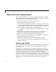
Smoothing Data Savitzky-Golay Filtering Savitzky-Golay filtering can be thought of as a generalized moving average. You derive the filter coefficients by performing an unweighted linear least squares fit using a polynomial of a given degree. For this reason, a Savitzky-Golay filter is also called a digital smoothing polynomial filter or a least squares smoothing filter. Note that a higher degree polynomial makes it possible to achieve a high level of smoothing without attenuation of data features.
2 Importing, Viewing, and Preprocessing Data Savitzky−Golay Smoothing 80 noisy data 60 40 20 0 1 2 3 4 5 6 7 8 (a) 80 data S−G quadratic 60 40 20 0 1 2 3 4 5 6 7 8 (b) 80 data S−G quartic 60 40 20 0 1 2 3 4 5 6 7 8 (c) Plot (a) shows the noisy data. To more easily compare the smoothed results, plots (b) and (c) show the data without the added noise. Plot (b) shows the result of smoothing with a quadratic polynomial. Notice that the method performs poorly for the narrow peaks.
Smoothing Data Example: Smoothing Data This example smooths the ENSO data set using the moving average, lowess, loess, and Savitzky-Golay methods with the default span. As shown below, the data appears noisy. Smoothing might help you visualize patterns in the data, and provide insight toward a reasonable approach for parametric fitting. Because the data appears noisy, smoothing might help uncover its structure.
2 Importing, Viewing, and Preprocessing Data The Smooth pane shown below displays all the new data sets generated by smoothing the original ENSO data set. Whenever you smooth a data set, a new data set of smoothed values is created. The smoothed data sets are automatically displayed in the Curve Fitting Tool. You can also display a single data set graphically and numerically by clicking the View button. A new data set composed of smoothed values is created from the original data set.
Smoothing Data Use the Plotting GUI to display only the data sets of interest. As shown below, the periodic structure of the ENSO data set becomes apparent when it is smoothed using a moving average filter with the default span. Not surprisingly, the uncovered structure is periodic, which suggests that a reasonable parametric model should include trigonometric functions. Display only the data set created with the moving average method.
2 Importing, Viewing, and Preprocessing Data Saving the Results By clicking the Save to workspace button, you can save a smoothed data set as a structure to the MATLAB workspace. This example saves the moving average results contained in the enso (ma) data set. The saved structure contains the original predictor data x and the smoothed data y.
Excluding and Sectioning Data Excluding and Sectioning Data If there is justification, you might want to exclude part of a data set from a fit. Typically, you exclude data so that subsequent fits are not adversely affected. For example, if you are fitting a parametric model to measured data that has been corrupted by a faulty sensor, the resulting fit coefficients will be inaccurate.
2 Importing, Viewing, and Preprocessing Data You mark data to be excluded from a fit with the Exclude GUI, which you open from the Curve Fitting Tool. The GUI is shown below followed by a description of its features. Exclusion rule. Exclude individual data points. Exclude data sections by domain or range. Exclusion Rule • Exclusion rule name — Specify the name of the exclusion rule that identifies the data points to be excluded from subsequent fits.
Excluding and Sectioning Data Exclude Individual Data Points • Select data set — Select the data set from which data points will be marked as excluded. You must select a data set to exclude individual data points. • Exclude graphically — Open a GUI that allows you to exclude individual data points graphically. Individually excluded data points are marked by an “x” in the GUI, and are automatically identified in the Check to exclude point table.
2 Importing, Viewing, and Preprocessing Data by a particular distribution, which is often assumed to be Gaussian. The statistical nature of the data implies that it contains random variations along with a deterministic component. data = deterministic component + random component However, your data set might contain one or more data points that are nonstatistical in nature, or are described by a different statistical distribution.
Excluding and Sectioning Data Two types of influential data points are shown below for generated data. Also shown are cubic polynomial fits and a robust fit that is resistant to outliers. Influential Data Points 150 data cubic fit 100 These outliers adversely affect the fit. 50 0 1 2 3 4 5 6 7 8 9 10 (a) 150 data cubic fit 100 These data points are consistent with the model.
2 Importing, Viewing, and Preprocessing Data Sectioning Sectioning involves specifying a range of response data or a range of predictor data to exclude. You might want to section a data set because different parts of the data set are described by different models or many contiguous data points are corrupted by noise, large systematic errors, and so on.
Excluding and Sectioning Data Two examples of sectioning by domain are shown below for generated data. Sectioning Data 400 data linear fit cubic fit 200 0 −200 −400 −600 −800 1000 1200 0 2 4 6 8 10 (a) 12 14 16 18 20 400 data linear fit cubic fit 200 0 −200 −400 −600 −800 1000 1200 0 2 4 6 8 10 (b) 12 14 16 18 20 Plot (a) shows the data set sectioned by fit type. The left section is fit with a linear polynomial, while the right section is fit with a cubic polynomial.
2 Importing, Viewing, and Preprocessing Data Example: Excluding and Sectioning Data This example modifies the ENSO data set to illustrate excluding and sectioning data. First, copy the ENSO response data to a new variable and add two outliers that are far removed from the bulk of the data. rand('state',0) yy = pressure; yy(ceil(length(month)*rand(1))) = mean(pressure)*2.5; yy(ceil(length(month)*rand(1))) = mean(pressure)*3.
Excluding and Sectioning Data To mark data points for exclusion in the GUI, place the mouse cursor over the data point and left-click. The excluded data point is marked with a red X. To include an excluded data point, right-click the data point or select the Include Them radio button and left-click. Included data points are marked with a blue circle.
2 Importing, Viewing, and Preprocessing Data The Exclude GUI for this example is shown below. Individual data points marked for exclusion. Data points outside the specified domain are marked for exclusion. To save the exclusion rule, click the Create exclusion rule button. To exclude the data from a fit, you must select the exclusion rule from the Fitting GUI.
Excluding and Sectioning Data Viewing the Exclusion Rule To view the exclusion rule, select an existing exclusion rule name and click the View button. The View Exclusion Rule GUI shown below displays the modified ENSO data set and the excluded data points, which are grayed in the table. The excluded data points are grayed in the table. Example: Sectioning Periodic Data For all parametric equations, the toolbox provides coefficient starting values.
2 Importing, Viewing, and Preprocessing Data the amplitude starting point is reasonably close to the expected value, but the frequency and phase constant are not, which produces a poor fit. The amplitude starting point is reasonably close to the expected value, but the frequency and phase constant are not.
Excluding and Sectioning Data To produce a reasonable fit, follow these steps: 1 Create an exclusion rule that includes one or two periods, and excludes the remaining data. As shown below, an exclusion rule is created graphically by using the selection rubber band to exclude all data points outside the first period. The exclusion rule is named 1Period. Exclude data graphically. Use the selection rubber band to exclude data points outside the first period.
2 Importing, Viewing, and Preprocessing Data 2 Create a new fit using the single-term sine equation with the exclusion rule 1Period applied. The fit looks reasonable throughout the entire data set. However, because the global fit was based on a small fraction of data, goodness of fit statistics will not provide much insight into the fit quality. Apply exclusion rule to the single-term exponential fit.
Excluding and Sectioning Data 3 Fit the entire data set using the fitted coefficient values from the previous step as starting values. The Fitting GUI, Fit Options GUI, and Curve Fitting Tool are shown below. Both the numerical and graphical fit results indicate a reasonable fit. The coefficient starting values are given by the previous fit results.
2 Importing, Viewing, and Preprocessing Data Additional Preprocessing Steps Additional preprocessing steps not available through the Curve Fitting Toolbox GUIs include • Transforming the response data • Removing Infs, NaNs, and outliers Transforming the Response Data In some circumstances, you might want to transform the response data. Common transformations include the logarithm ln(y), and power functions such as y1/2, y-1, and so on.
Additional Preprocessing Steps There are several disadvantages associated with performing transformations: • For the log transformation, negative response values cannot be processed. • For all transformations, the basic assumption that the residual variance is constant is violated. To avoid this problem, you could plot the residuals on the transformed scale.
2 Importing, Viewing, and Preprocessing Data Selected Bibliography [1] Cleveland, W.S., “Robust Locally Weighted Regression and Smoothing Scatterplots,” Journal of the American Statistical Association, Vol. 74, pp. 829-836, 1979. [2] Cleveland, W.S. and S.J. Devlin, “Locally Weighted Regression: An Approach to Regression Analysis by Local Fitting,” Journal of the American Statistical Association, Vol. 83, pp. 596-610, 1988. [3] Chambers, J., W.S. Cleveland, B. Kleiner, and P.
3 Fitting Data Curve fitting refers to fitting curved lines to data. The curved line comes from regression techniques, a spline calculation, or interpolation. The data can be measured from a sensor, generated from a simulation, historical, and so on. The goal of curve fitting is to gain insight into your data.
3 Fitting Data The Fitting Process You fit data using the Fitting GUI. To open the Fitting GUI, click the Fitting button from the Curve Fitting Tool. The Fitting GUI is shown below for the census data described in “Getting Started with the Curve Fitting Toolbox” on page 1-1, followed by the general steps you use when fitting any data set. 1. Select a data set and specify a fit name. 2. Select an exclusion rule. 3. Select a fit type, select fit options, fit the data, and evaluate the goodness of fit. 4.
The Fitting Process 1 Select a data set and fit name. - Select the name of the current fit. When you click New fit or Copy fit, a default fit name is automatically created in the Fit name field. You can specify a new fit name by editing this field. - Select the name of the current data set from the Data set list. All imported and smoothed data sets are listed. 2 Select an exclusion rule. If you want to exclude data from a fit, select an exclusion rule from the Exclusion rule list.
3 Fitting Data Parametric Fitting Parametric fitting involves finding coefficients (parameters) for one or more models that you fit to data. The data is assumed to be statistical in nature and is divided into two components: a deterministic component and a random component. data = deterministic component + random component The deterministic component is given by the fit and the random component is often described as error associated with the data.
Parametric Fitting Basic Assumptions About the Error When fitting data that contains random variations, there are two important assumptions that are usually made about the error: • The error exists only in the response data, and not in the predictor data. • The errors are random and follow a normal (Gaussian) distribution with zero mean and constant variance, σ2. The second assumption is often expressed as 2 error ∼ N ( 0, σ ) The components of this expression are described below.
3 Fitting Data The Least Squares Fitting Method The Curve Fitting Toolbox uses the method of least squares when fitting data. The fitting process requires a model that relates the response data to the predictor data with one or more coefficients. The result of the fitting process is an estimate of the “true” but unknown coefficients of the model. To obtain the coefficient estimates, the least squares method minimizes the summed square of residuals.
Parametric Fitting To solve this equation for the unknown coefficients p1 and p2, you write S as a system of n simultaneous linear equations in two unknowns. If n is greater than the number of unknowns, then the system of equations is overdetermined. n ∑ ( y i – ( p 1 xi + p 2 ) ) S = 2 i=1 Because the least squares fitting process minimizes the summed square of the residuals, the coefficients are determined by differentiating S with respect to each parameter, and setting the result equal to zero.
3 Fitting Data Solving for b2 using the b1 value 1 b 2 = --- n ∑ yi – b1 ∑ xi As you can see, estimating the coefficients p1 and p2 requires only a few simple calculations. Extending this example to a higher degree polynomial is straightforward although a bit tedious. All that is required is an additional normal equation for each linear term added to the model. In matrix form, linear models are given by the formula y = Xβ + ε where • y is an n-by-1 vector of responses.
Parametric Fitting where XT is the transpose of the design matrix X. Solving for b, –1 T T b = (X X) X y In MATLAB, you can use the backslash operator to solve a system of simultaneous linear equations for unknown coefficients. Because inverting XTX can lead to unacceptable rounding errors, MATLAB uses QR decomposition with pivoting, which is a very stable algorithm numerically.
3 Fitting Data where wi are the weights. The weights determine how much each response value influences the final parameter estimates. A high-quality data point influences the fit more than a low-quality data point. Weighting your data is recommended if the weights are known, or if there is justification that they follow a particular form.
Parametric Fitting The weights you supply should transform the response variances to a constant value. If you know the variances of your data, then the weights are given by wi = 1 ⁄ σ 2 If you don’t know the variances, you can approximate the weights using an equation such as n 2 1 w i = --( yi – y ) n i=1 –1 ∑ This equation works well if your data set contains replicates. In this case, n is the number of sets of replicates. However, the weights can vary greatly.
3 Fitting Data the line get reduced weight. Points that are farther from the line than would be expected by random chance get zero weight. For most cases, the bisquare weight scheme is preferred over LAR because it simultaneously seeks to find a curve that fits the bulk of the data using the usual least squares approach, and it minimizes the effect of outliers.
Parametric Fitting 4 If the fit converges, then you are done. Otherwise, perform the next iteration of the fitting procedure by returning to the first step. The plot shown below compares a regular linear fit with a robust fit using bisquare weights. Notice that the robust fit follows the bulk of the data and is not strongly influenced by the outliers.
3 Fitting Data Nonlinear Least Squares The Curve Fitting Toolbox uses the nonlinear least squares formulation to fit a nonlinear model to data. A nonlinear model is defined as an equation that is nonlinear in the coefficients, or a combination of linear and nonlinear in the coefficients. For example, Gaussians, ratios of polynomials, and power functions are all nonlinear. In matrix form, nonlinear models are given by the formula y = f ( X, β ) + ε where • y is an n-by-1 vector of responses.
Parametric Fitting 3 Adjust the coefficients and determine whether the fit improves. The direction and magnitude of the adjustment depend on the fitting algorithm. The toolbox provides these algorithms: - Trust-region — This is the default algorithm and must be used if you specify coefficient constraints. It can solve difficult nonlinear problems more efficiently than the other algorithms and it represents an improvement over the popular Levenberg-Marquardt algorithm.
3 Fitting Data Library Models The parametric library models provided by the Curve Fitting Toolbox are described below. Exponentials The toolbox provides a one-term and a two-term exponential model. y = ae y = ae bx bx + ce dx Exponentials are often used when the rate of change of a quantity is proportional to the initial amount of the quantity. If the coefficient associated with e is negative, y represents exponential decay. If the coefficient is positive, y represents exponential growth.
Parametric Fitting For more information about the Fourier series, refer to “Fourier Analysis and the Fast Fourier Transform” in the MATLAB documentation. For an example that fits the ENSO data to a custom Fourier series model, refer to “General Equation: Fourier Series Fit” on page 3-52.
3 Fitting Data conversion for a Type J thermocouple in the 0o to 760o temperature range is described by a seventh-degree polynomial. Note If you do not require a global parametric fit and want to maximize the flexibility of the fit, piecewise polynomials might provide the best approach. Refer to “Nonparametric Fitting” on page 3-68 for more information.
Parametric Fitting Rationals Rational models are defined as ratios of polynomials and are given by n+1 ∑ pi x n+1–i i=1 y = ------------------------------------------m x m ∑ qi x + m–i i=1 where n is the degree of the numerator polynomial and 0 ≤ n ≤ 5 , while m is the degree of the denominator polynomial and 1 ≤ m ≤ 5 . Note that the coefficient m associated with x is always 1. This makes the numerator and denominator unique when the polynomial degrees are the same.
3 Fitting Data difference is that the sum of sines equation includes the phase constant, and does not include a DC offset term. Weibull Distribution The Weibull distribution is widely used in reliability and life (failure rate) data analysis. The toolbox provides the two-parameter Weibull distribution y = abx b – 1 – ax b e where a is the scale parameter and b is the shape parameter.
Parametric Fitting You create custom equations with the Create Custom Equation GUI. The GUI contains two panes: a pane for creating linear equations and a pane for creating general (nonlinear) equations. These panes are described below. Linear Equations Linear equations are defined as equations that are linear in the parameters. For example, the polynomial library equations are linear. The Linear Equations pane is shown below followed by a description of its parameters.
3 Fitting Data • Equation — The custom equation. • Equation name — The name of the equation. By default, the name is automatically updated to be identical to the custom equation given by Equation. If you override the default, the name is no longer automatically updated. General Equations General (nonlinear) equations are defined as equations that are nonlinear in the parameters, or are a combination of linear and nonlinear in the parameters. For example, the exponential library equations are nonlinear.
Parametric Fitting • Equation name — The name of the equation. By default, the name is automatically updated to be identical to the custom equation given by Equation. If you override the default, the name is no longer automatically updated. Note that even if you define a linear equation, a nonlinear fitting procedure is used. Although this is allowed by the toolbox, it is an inefficient process and can result in less than optimal fitted coefficients.
3 Fitting Data Fitting Method and Algorithm • Method — The fitting method. The method is automatically selected based on the library or custom model you use. For linear models, the method is LinearLeastSquares. For nonlinear models, the method is NonlinearLeastSquares. • Robust — Specify whether to use the robust least squares fitting method. The values are - Off — Do not use robust fitting (default). - On — Fit with default robust method (bisquare weights).
Parametric Fitting • TolFun — Termination tolerance used on stopping conditions involving the function (model) value. The default value is 10-6. • TolX — Termination tolerance used on stopping conditions involving the coefficients. The default value is 10-6. Coefficient Parameters • Unknowns — Symbols for the unknown coefficients to be fitted. • StartPoint — The coefficient starting values. The default values depend on the model.
3 Fitting Data Default Coefficient Parameters The default coefficient starting points and constraints for library and custom models are given below. If the starting points are optimized, then they are calculated heuristically based on the current data set. Random starting points are defined on the interval [0,1] and linear models do not require starting points. If a model does not have constraints, the coefficients have neither a lower bound nor an upper bound.
Parametric Fitting Evaluating the Goodness of Fit After fitting data with one or more models, you should evaluate the goodness of fit. A visual examination of the fitted curve displayed in the Curve Fitting Tool should be your first step. Beyond that, the toolbox provides these goodness of fit measures for both linear and nonlinear parametric fits: • Residuals • Goodness of fit statistics • Confidence and prediction bounds You can group these measures into two types: graphical and numerical.
3 Fitting Data Mathematically, the residual for a specific predictor value is the difference between the response value y and the predicted response value ŷ . r = y – ŷ Assuming the model you fit to the data is correct, the residuals approximate the random errors. Therefore, if the residuals appear to behave randomly, it suggests that the model fits the data well. However, if the residuals display a systematic pattern, it is a clear sign that the model fits the data poorly.
Parametric Fitting A graphical display of the residuals for a second-degree polynomial fit is shown below. The model includes only the quadratic term, and does not include a linear or constant term. 12 Data Quadratic Fit 10 8 6 4 2 0 0 1 2 3 4 5 6 7 8 9 10 11 2 3 4 5 6 7 8 9 10 11 Residuals 3 2 1 0 −1 −2 −3 0 1 The residuals are systematically positive for much of the data range indicating that this model is a poor fit for the data.
3 Fitting Data For the current fit, these statistics are displayed in the Results list box in the Fit Editor. For all fits in the current curve-fitting session, you can compare the goodness of fit statistics in the Table of fits. Sum of Squares Due to Error. This statistic measures the total deviation of the response values from the fit to the response values. It is also called the summed square of residuals and is usually labeled as SSE.
Parametric Fitting If you increase the number of fitted coefficients in your model, R-square might increase although the fit may not improve. To avoid this situation, you should use the degrees of freedom adjusted R-square statistic described below. Note that it is possible to get a negative R-square for equations that do not contain a constant term.
3 Fitting Data Confidence and Prediction Bounds With the Curve Fitting Toolbox, you can calculate confidence bounds for the fitted coefficients, and prediction bounds for new observations or for the fitted function. Additionally, for prediction bounds, you can calculate simultaneous bounds, which take into account all predictor values, or you can calculate nonsimultaneous bounds, which take into account only individual predictor values.
Parametric Fitting Calculating and Displaying Confidence Bounds. The confidence bounds for fitted coefficients are given by C = b±t S where b are the coefficients produced by the fit, t is the inverse of Student’s T cumulative distribution function, and S is a vector of the diagonal elements from the covariance matrix of the coefficient estimates, (XTX)-1s2. X is the design matrix, XT is the transpose of X, and s2 is the mean squared error.
3 Fitting Data The nonsimultaneous prediction bounds for a new observation at the predictor value x are given by 2 P n, o = ŷ ± t s + xSx' where s2 is the mean squared error, t is the inverse of Student’s T cumulative distribution function, and S is the covariance matrix of the coefficient estimates, (XTX)-1s2. Note that x is defined as a row vector of the Jacobian evaluated at a specified predictor value.
Parametric Fitting To understand the quantities associated with each type of prediction interval, recall that the data, fit, and residuals (random errors) are related through the formula data = fit + residuals Suppose you plan to take a new observation at the predictor value xn+1. Call the new observation yn+1(xn+1) and the associated error en+1. Then yn+1(xn+1) satisfies the equation yn + 1 ( xn + 1 ) = f ( xn + 1 ) + en + 1 where f(xn+1) is the true but unknown function you want to estimate at xn+1.
3 Fitting Data are wider than the fitted function intervals because of the additional uncertainty in predicting a new response value (the fit plus random errors). Nonsimultaneous bounds for function Nonsimultaneous bounds for observation 2.5 2.5 data fitted curve prediction bounds 2 data fitted curve prediction bounds 2 1.5 y y 1.5 1 1 0.5 0.5 0 0 0 2 4 6 8 −0.5 10 0 2 4 x 6 8 10 x Simultaneous bounds for function Simultaneous bounds for observation 2.5 2.
Parametric Fitting Example: Evaluating the Goodness of Fit This example fits several polynomial models to generated data and evaluates the goodness of fit. The data is cubic and includes a range of missing values. rand('state',0) x = [1:0.1:3 9:0.1:10]'; c = [2.5 -0.5 1.3 -0.1]; y = c(1) + c(2)*x + c(3)*x.^2 + c(4)*x.^3 + (rand(size(x))-0.5); After you import the data, fit it using a cubic polynomial and a fifth degree polynomial. The data, fits, and residuals are shown below.
3 Fitting Data The numerical fit results are shown below. The cubic fit coefficients are accurately known. The quintic fit coefficients are not accurately known. As expected, the fit results for poly3 are reasonable because the generated data is cubic. The 95% confidence bounds on the fitted coefficients indicate that they are acceptably accurate. However, the 95% confidence bounds for poly5 indicate that the fitted coefficients are not known accurately. The goodness of fit statistics are shown below.
Parametric Fitting The 95% nonsimultaneous prediction bounds for new observations are shown below. To display prediction bounds in the Curve Fitting Tool, select the View->Prediction Bounds menu item. Alternatively, you can view prediction bounds for the function or for new observations using the Analysis GUI. The prediction bounds for poly3 indicate that new observations can be predicted accurately throughout the entire data range. This is not the case for poly5.
3 Fitting Data Therefore, you would conclude that more data must be collected before you can make accurate predictions using a fifth-degree polynomial. In conclusion, you should examine all available goodness of fit measures before deciding on the best fit. A graphical examination of the fit and residuals should always be your initial approach. However, some fit characteristics are revealed only through numerical fit results, statistics, and prediction bounds.
Parametric Fitting Example: Rational Fit This example fits measured data using a rational model. The data describes the coefficient of thermal expansion for copper as a function of temperature in degrees Kelvin. To get started, load the thermal expansion data from the file hahn1.mat, which is provided with the toolbox. load hahn1 The workspace now contains two new variables, temp and thermex: • temp is a vector of temperatures in degrees Kelvin.
3 Fitting Data As you can see by examining the shape of the data, a reasonable initial choice for the rational model is quadratic/quadratic. The Fitting GUI configured for this equation is shown below. Begin the fitting process with a quadratic/quadratic rational fit.
Parametric Fitting The data, fit, and residuals are shown below. The fit clearly misses some of the data. The residuals show a strong pattern indicating a better fit is possible. The fit clearly misses the data for the smallest and largest predictor values. Additionally, the residuals show a strong pattern throughout the entire data set indicating that a better fit is possible.
3 Fitting Data For the next fit, try a cubic/cubic equation. The data, fit, and residuals are shown below. The fit exhibits several discontinuities around the zeros of the denominator. The numerical results shown below indicate that the fit did not converge. The fit did not converge, which indicates that the model might be a poor choice for the data.
Parametric Fitting Although the message in the Results window indicates that you might improve the fit if you increase the maximum number of iterations, a better choice at this stage of the fitting process is to use a different rational equation because the current fit contains several discontinuities. These discontinuities are due to the function blowing up at predictor values that correspond to the zeros of the denominator. As the next try, fit the data using a cubic/quadratic equation.
3 Fitting Data Example: Fitting with Custom Equations You can define your own equations with the Create Custom Equation GUI. You open this GUI one of two ways: • From the Curve Fitting Tool, select Tools->Custom Equation. • From the Fitting GUI, select Custom Equations from the Type of fit list, then click the New Equation button. The Create Custom Equation GUI contains two panes: one for creating linear custom equations and one for creating general (nonlinear) custom equations.
Parametric Fitting It is sometimes useful to describe a variable expressed as a function of angle in terms of Legendre polynomials ∞ y( x) = ∑ an Pn ( x ) n=0 where Pn(x) is a Legendre polynomial of degree n, x is cos(θα), and an are the coefficients of the fit. Refer to MATLAB’s legendre function for information about generating Legendre polynomials.
3 Fitting Data The first step is to load the 12C alpha-emission data from the file carbon12alpha.mat, which is provided with the toolbox. load carbon12alpha The workspace now contains two new variables, angle and counts: • angle is a vector of angles (in radians) ranging from 10o to 240o in 10o increments. • counts is a vector of raw alpha particle counts that correspond to the emission angles in angle. Import these two variables into the Curve Fitting Toolbox and name the data set C12Alpha.
Parametric Fitting Fit the data using a fourth-degree Legendre polynomial with only even terms: 1 2 1 4 2 y 1 ( x ) = a 0 + a 2 --- ( 3x – 1 ) + a 4 --- ( 35x – 30x + 3 ) 2 8 Because the Legendre polynomials depend only on the predictor variable and constants, you use the Linear Equations pane on the Create Custom Equation GUI. This pane is shown below for the model given by y1(x). Note that because angle is given in radians, the argument of the Legendre terms is given by cos(θα).
3 Fitting Data The fit and residuals are shown below. The fit appears to follow the trend of the data well, while the residuals appear to be randomly distributed and do not exhibit any systematic behavior. The numerical fit results are shown below. The 95% confidence bounds indicate that the coefficients associated with P0(x) and P4(x) are known fairly accurately, but that the P2(x) coefficient has a relatively large uncertainty.
Parametric Fitting To confirm the theoretical argument that the alpha-emission data is best described by a fourth-degree Legendre polynomial with only even terms, fit the data using both even and odd terms: 1 3 y 2 ( x ) = y 1 ( x ) + a 1 x + a3 --- ( 5x – 3x ) 2 The Linear Equations pane of the Create Custom Equation GUI is shown below for the model given by y2(x). Create a custom linear equation using even and odd Legendre terms up to fourth degree. Click Add a term to add the odd Legendre terms.
3 Fitting Data General Equation: Fourier Series Fit This example fits the ENSO data using several custom nonlinear equations. The ENSO data consists of monthly averaged atmospheric pressure differences between Easter Island and Darwin, Australia. This difference drives the trade winds in the southern hemisphere.
Parametric Fitting Note that the toolbox includes the Fourier series as a nonlinear library equation. However, the library equation does not meet the needs of this example because its terms are defined as fixed multiples of the fundamental frequency w. Refer to “Fourier Series” on page 3-16 for more information. The numerical results shown below indicate that the fit does not describe the data well. In particular, the fitted value for c1 is unreasonably small.
3 Fitting Data The fit, residuals, and numerical results are shown below. The fit for one cycle. The residuals indicate that at least one more cycle exists. The numerical results indicate a 12 month cycle. The fit appears to be reasonable for some of the data points but clearly does not describe the entire data set very well. As predicted, the numerical results indicate a cycle of approximately 12 months.
Parametric Fitting The fit, residuals, and numerical results are shown below. The fit for two cycles. The residuals indicate that one more cycle might exist. The numerical results indicate an additional 22 month cycle. The fit appears to be reasonable for most of the data points. However, the residuals indicate that you should include another cycle to the fit equation.
3 Fitting Data The fit, residuals, and numerical results are shown below. The fit for three cycles. The residuals appear fairly random for most of the data set. The numerical results indicate 12, 22, and 44 month cycles. The fit is an improvement over the previous two fits, and appears to account for most of the cycles present in the ENSO data set.
Parametric Fitting General Equation: Gaussian Fit with Exponential Background This example fits two poorly resolved Gaussian peaks on a decaying exponential background using a general (nonlinear) custom model. To get started, load the data from the file gauss3.mat, which is provided with the toolbox. load gauss3 The workspace now contains two new variables, xpeak and ypeak: • xpeak is a vector of predictor values. • ypeak is a vector of response values.
3 Fitting Data The data, fit, and numerical fit results are shown below. Clearly, the fit is poor. Because the starting points are randomly selected, your initial fit results might differ from the results shown here.
Parametric Fitting The results include this warning message. Fit computation did not converge: Maximum number of function evaluations exceeded. Increasing MaxFunEvals (in fit options) may allow for a better fit, or the current equation may not be a good model for the data. To improve the fit for this example, specify reasonable starting points for the coefficients.
3 Fitting Data The data, fit, residuals, and numerical results are shown below.
Parametric Fitting Example: Robust Fit This example fits data that is assumed to contain one outlier. The data consists of the 2000 United States presidential election results for the state of Florida. The fit model is a first degree polynomial and the fit method is robust linear least squares with bisquare weights.
3 Fitting Data To create a first-degree polynomial equation with zero offset, you must create a custom linear equation. As described in “Example: Fitting with Custom Equations” on page 3-46, you can create a custom equation using the Fitting GUI by selecting Custom Equations from the Type of fit list, and then clicking the New Equation button. The Linear Equations pane of the Create Custom Equation GUI is shown below. Create a first-degree polynomial with zero offset. Clear this check box.
Parametric Fitting The Exclude GUI is shown below. Mark the absentee votes to be excluded. The exclusion rule is named AbsenteeVotes. You use the Fitting GUI to associate an exclusion rule with the data set to be fit. For each data set, perform a robust fit with bisquare weights using the FlaElection equation defined above. For comparison purposes, also perform a regular linear least squares fit.
3 Fitting Data The Fit Editor and the Fit Options GUI are shown below for a robust fit. Associate the excluded absentee votes with the fit. Choose robust fitting with bisquare weights. Open the Fit Options GUI. The data, robust and regular least squares fits, and residuals for the buchanan vs. bush data set are shown below. The data tip shows that Buchanan received 3411 votes in Palm Beach County. The Palm Beach County residual is very large. The Miami/Dade County residual is also very large.
Parametric Fitting The graphical results show that the linear model is reasonable for the majority of data points, and the residuals appear to be randomly scattered around zero. However, two residuals stand out. The largest residual corresponds to Palm Beach County. The other residual is at the largest predictor value, and corresponds to Miami/Dade County. The numerical results are shown below. The inverse slope of the robust fit indicates that Buchanan should receive one vote for every 197.4 Bush votes.
3 Fitting Data Again, the graphical results show that the linear model is reasonable for the majority of data points, and the residuals appear to be randomly scattered around zero. However, three residuals stand out. The largest residual corresponds to Palm Beach County. The other residuals are at the two largest predictor values, and correspond to Miami/Dade County and Broward County. The numerical results are shown below.
Parametric Fitting The margin of victory for George Bush is given by margin = sum(bush)–sum(gore) margin = 537 Therefore, the voter intention comes into play because in both cases, the margin of victory is less than the excess Buchanan votes.
3 Fitting Data Nonparametric Fitting In some cases, you are not concerned about extracting or interpreting fitted parameters. Instead, you might simply want to draw a smooth curve through your data. Fitting of this type is called nonparametric fitting. The Curve Fitting Toolbox supports these nonparametric fitting methods: • Interpolants — Estimate values that lie between known data points. • Smoothing spline — Create a smooth curve through the data.
Nonparametric Fitting The type of interpolant you should use depends on the characteristics of the data being fit, the required smoothness of the curve, speed considerations, postfit analysis requirements, and so on. The linear and nearest neighbor methods are fast, but the resulting curves are not very smooth. The cubic spline and shape-preserving methods are slower, but the resulting curves are often very smooth. For example, the nuclear reaction data from the file carbon12alpha.
3 Fitting Data Note Goodness of fit statistics, prediction bounds, and weights are not defined for interpolants. Additionally, the fit residuals are always zero (within computer precision) because interpolants pass through the data points. Interpolants are defined as piecewise polynomials because the fitted curve is constructed from many “pieces.” For cubic spline and PCHIP interpolation, each piece is described by four coefficients, which are calculated using a cubic (third-degree) polynomial.
Nonparametric Fitting parameter, you can consider these fits to be parametric. However, smoothing splines are also piecewise polynomials like cubic spline or shape-preserving interpolants and are considered a nonparametric fit type in this guide. Note The smoothing spline algorithm used by the Curve Fitting Toolbox is based on the csaps function included with the Spline Toolbox. Refer to the csaps reference pages for detailed information about smoothing splines.
3 Fitting Data Example: Nonparametric Fit This example fits the following data using a cubic spline interpolant and several smoothing splines. rand('state',0); x = (4*pi)*[0 1 rand(1,25)]; y = sin(x) + .2*(rand(size(x))-.5); As shown below, you can fit the data with a cubic spline by selecting Interpolant from the Type of fit list. The results shown below indicate that goodness of fit statistics are not defined for interpolants.
Nonparametric Fitting As shown below, you can fit the data with a smoothing spline by selecting Smoothing Spline in the Type of fit list. The default smoothing parameter is based on the data set you fit. The level of smoothness is given by the Smoothing Parameter. The default smoothing parameter value depends on the data set, and is automatically calculated by the toolbox after you click the Apply button.
3 Fitting Data The data and fits are shown below. The default abscissa scale was increased to show the fit behavior beyond the data limits. You change the axes limits with Tools->Axes Limit Control menu item. The cubic spline and default smoothing spline results are similar for interior points. The cubic spline and default smoothing spline results diverge at the end points. The default smoothing parameter produces the smoothest result.
Selected Bibliography Selected Bibliography [1] Draper, N.R and H. Smith, Applied Regression Analysis, 3rd Ed., John Wiley & Sons, New York, 1998. [2] Bevington, P.R. and D.K. Robinson, Data Reduction and Error Analysis for the Physical Sciences, 2nd Ed., WCB/McGraw-Hill, Boston, 1992. [3] Daniel, C. and F.S. Wood, Fitting Equations to Data, John Wiley & Sons, New York, 1980. [4] Branch, M.A., T.F. Coleman, and Y.
3 Fitting Data 3-76
4 Function Reference This chapter describes the toolbox M-file functions that you use directly. A number of other M-file helper functions are provided with this toolbox to support the functions listed below. These helper functions are not documented because they are not intended for direct use. Functions – By Category (p. 4-78) Contains a series of tables that group functions by category Functions – Alphabetical List (p.
4 Function Reference Functions – By Category Fitting Data cfit Create a cfit object fit Fit data using a library or custom model, a smoothing spline, or an interpolant fitoptions Create or modify a fit options object fittype Create a fit type object Getting Information and Help cflibhelp Display information about library models, splines, and interpolants disp Display descriptive information for Curve Fitting Toolbox objects Getting and Setting Properties get Return properties for a fit option
Functions – By Category Postprocessing Data confint Compute confidence bounds for fitted coefficients differentiate Differentiate a fit result object integrate Integrate a fit result object predint Compute prediction bounds for new observations or for the function General Purpose cftool Open the Curve Fitting Tool datastats Return descriptive statistics about the data feval Evaluate a fit result object or a fit type object plot Plot data, fit, prediction bounds, outliers, and residuals 4-79
4 Function Reference Functions – Alphabetical List This section contains detailed descriptions of all toolbox functions. Each function reference page contains some or all of this information: • The function name • The purpose of the function • The function syntax All valid input argument and output argument combinations are shown. In some cases, an ellipsis (. . .) is used for the input arguments. This means that all preceding input argument combinations are valid for the specified output argument(s).
cfit Purpose 4cfit Create a cfit object Syntax fmodel = cfit(ftype,coef1,coef2,...) Arguments ftype A fit type object representing a custom or library model. coef1,coef2,... The model coefficients. fmodel Description The cfit object. fmodel = cfit(ftype,coef1,coef2,...) creates the cfit object fmodel based on the custom or library model specified by ftype, and with the coefficients specified by coef1, coef2, and so on. You create ftype with the fittype function.
cflibhelp Purpose Syntax 4cflibhelp Display information about library models, splines, and interpolants cflibhelp cflibhelp group Arguments group Description cflibhelp displays the names, equations, and descriptions for all the fit types The name of the fit type group. in the curve fitting library. You can use the fit type name as an input parameter to the fit, cfit, and fittype functions. cflibhelp group displays the names, equations, and descriptions for the fit type group specified by group.
cflibhelp Example Display the names and descriptions for the spline fit type group. cflibhelp spline SPLINES SPLINETYPE DESCRIPTION cubicspline smoothingspline cubic interpolating spline smoothing spline Display the model names and equations for the polynomial fit type group. cflibhelp polynomial POLYNOMIAL MODELS MODELNAME poly1 poly2 poly3 ... poly9 See Also EQUATION Y = p1*x+p2 Y = p1*x^2+p2*x+p3 Y = p1*x^3+p2*x^2+...+p4 Y = p1*x^9+p2*x^8+...
cftool Purpose Syntax Arguments Description 4cftool Open the Curve Fitting Tool cftool cftool(xdata,ydata) xdata A vector of predictor data. ydata A vector of response data. cftool opens the Curve Fitting Tool. cftool(xdata,ydata) opens the Curve Fitting Tool with predictor data specified by xdata and response data specified by ydata. xdata and ydata must be vectors of the same size. Infs and NaNs are ignored because you cannot fit data containing these values.
cftool The Curve Fitting Tool is shown below. The data is from the census MAT-file, and the fit is a quadratic polynomial. The residuals are shown as a line plot below the data and fit. The Curve Fitting Tool provides several features that facilitate data and fit exploration. Refer to “Viewing Data” on page 2-6 for a description of these features. By clicking the Data, Fitting, Exclude, Plotting, or Analysis buttons, you can open the associated GUIs, which are described below.
cftool The Data GUI The Data GUI allows you to • Import, preview, name, and delete data sets • Smooth noisy data The Data GUI is shown below with the census data loaded. Refer to Chapter 2, “Importing, Viewing, and Preprocessing Data” for more information about the Data GUI.
cftool The Fitting GUI The Fitting GUI allows you to • Fit data using a parametric or nonparametric equation • Examine and compare fit results including fitted coefficient values and goodness of fit statistics • Keep track of all the data sets and fits for the current session The Fitting GUI shown below displays the results of fitting the census data to a quadratic polynomial.
cftool The Exclude GUI The Exclude GUI allows you to create exclusion rules for a data set. An exclusion rule identifies data to be excluded while fitting. The excluded data can be individual data points, or a section of predictor or response data. The Exclude GUI shown below indicates that the first two data points of the census data are marked for exclusion, and that this exclusion rule is named exc1.
cftool The Analysis GUI The Analysis GUI allows you to • Evaluate (interpolate or extrapolate), differentiate, or integrate a fit • Plot the analysis results and the data set The Analysis GUI shown below displays the numerical results of extrapolating the census data from the year 2000 to the year 2050 in 10-year increments. Refer to “Analyzing the Fit” on page 1-15 for an example that uses the Analysis GUI.
confint Purpose Syntax Arguments Description 4confint Compute confidence bounds for fitted coefficients ci = confint(fresult) ci = confint(fresult,level) fresult A fit result object. level The confidence level. ci An array of confidence bounds. ci = confint(fresult) returns 95% confidence bounds to ci for the fit coefficients associated with fresult. fresult is the fit result object returned by the fit function. ci is a 2-by-n array where n is the number of coefficients associated with fresult.
confint Example Fit the census data to a second-degree polynomial. The display for fresult includes the 95% confidence bounds for the fitted coefficients. load census fresult = fit(cdate,pop,'poly2') fresult = Linear model Poly2: fresult(x) = p1*x^2 + p2*x + p3 Coefficients (with 95% confidence bounds): p1 = 0.006541 (0.006124, 0.006958) p2 = -23.51 (-25.09, -21.93) p3 = 2.113e+004 (1.964e+004, 2.262e+004) Calculate 95% confidence bounds for the fitted coefficients using confint. ci = confint(fresult,0.
datastats Purpose Syntax Arguments Description 4datastats Return descriptive statistics about the data xds = datastats(xdata) [xds,yds] = datastats(xdata,ydata) xdata A column vector of predictor data. ydata A column vector of response data. xds A structure containing descriptive statistics for xdata. yds A structure containing descriptive statistics for ydata. xds = datastats(xdata) returns statistics for xdata to the structure xds. The structure contains the fields shown below.
datastats Example Return data statistics for the census data. load census [xds,yds] = datastats(cdate,pop) xds = num: max: min: mean: median: range: std: 21 1990 1790 1890 1890 200 62.048 yds = num: max: min: mean: median: range: std: 21 248.7 3.9 85.729 62.9 244.8 78.
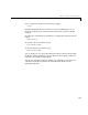
differentiate Purpose Syntax Arguments Description 4differentiate Differentiate a fit result object deriv1 = differentiate(fitresult,x) [deriv1,deriv2] = differentiate(...) fresult A fit result object. x A column vector of values at which fresult is differentiated. deriv1 A column vector of first derivatives. deriv2 A column vector of second derivatives. deriv1 = differentiate(fitresult,x) differentiates the fit result object fresult at the points specified by x and returns the result to deriv1.
differentiate Example Create a noisy sine wave on the interval [0, 4π]. rand('state',0); x = linspace(0,4*pi,200)'; y = sin(x) + (rand(size(x))-0.5)*0.2; Create a custom fit type, and fit the data using reasonable starting values. ftype = fittype('a*sin(b*x)'); fopts = fitoptions('Method','Nonlinear','start',[1 1]); fit1 = fit(x,y,ftype,fopts); Calculate the first derivative for each value of x. deriv1 = differentiate(fit1,x); Plot the data, the fit to the data, and the first derivatives.
disp Purpose Syntax Arguments Description 4disp Display descriptive information for Curve Fitting Toolbox objects obj disp(obj) A Curve Fitting Toolbox object. obj obj or disp(obj) displays descriptive information for obj. You can create obj with the fit or cfit function, the fitoptions function, or the fittype function. Example The display for a custom fit type object is shown below.
disp Note that all fit types have the Normalize, Exclude, Weights, and Method fit options. Additional fit options are available depending on the Method value. For example, if Method is SmoothingSpline, the SmoothingParam fit option is available. The display for a fit result object is shown below. fresult = fit(cdate,pop,ftype,fopts) Warning: Start point not provided, choosing random start point. Maximum number of function evaluations exceeded.
excludedata Purpose 4excludedata Specify data to be excluded from a fit Syntax outliers = excludedata(xdata,ydata,’MethodName’,MethodValue) Arguments xdata A column vector of predictor data. ydata A column vector of response data. 'MethodName' The data exclusion method. Description MethodValue The value associated with MethodName. outliers A logical vector that defines data to be excluded from a fit.
excludedata Remarks You can combine data exclusion methods using logical operators. For example, to combine methods using the | (OR) operator outliers = excludedata(xdata,ydata,'indices',[3 5]); outliers = outliers|excludedata(xdata,ydata,'box',[1 10 0 90]); In some cases, you might want to use the ~ (NOT) operator to specify a box that contains all the data to exclude.
feval Purpose Syntax Arguments 4feval Evaluate a fit result object or a fit type object f = feval(fresult,x) f = feval(ftype,coef1,coef2,...,x) fresult A fit result object. x A column vector of values at which fresult or ftype is evaluated. ftype A fit type object. coef1,coef2,... The model coefficients assigned to ftype. f Description A column vector containing the result of evaluating fresult or ftype at x.
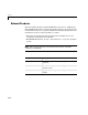
feval Create a fit result object and evaluate the object over a finer range in x. y = x.^2+(rand(size(x))-0.5); xx = (0:0.
fit Purpose Syntax Arguments Description 4fit Fit data using a library or custom model, a smoothing spline, or an interpolant fresult = fit(xdata,ydata,'ltype') fresult = fit(xdata,ydata,'ltype','PropertyName',PropertyValue,…) fresult = fit(xdata,ydata,'ltype',opts) fresult = fit(xdata,ydata,'ltype',...,'problem',values) fresult = fit(xdata,ydata,ftype,...) [fresult,gof] = fit(…) [fresult,gof,output] = fit(…) xdata A column vector of predictor data. ydata A column vector of response data.
fit fresult = fit(xdata,ydata,'ltype','PropertyName', PropertyValue,...) fits the data using the options specified by PropertyName and PropertyValue. You can display the fit options available for the specified library fit type with the fitoptions function. fresult = fit(xdata,ydata,'ltype',opts) fits the data using options specified by the fit options object opts. You create a fit options object with the fitoptions function. This is an alternative syntax to specifying property name/property value pairs.
fit example, the information returned for nonlinear least squares fits is given below. Remarks Field Description numobs Number of observations (response values). numparam Number of unknown parameters to fit. residuals Vector of residuals. Jacobian Jacobian matrix. exitflag Describes the exit condition. If exitflag > 0, the function converged to a solution. If exitflag = 0, the maximum number of function evaluations or iterations was exceeded.
fit Example Fit the census data with a second-degree polynomial library model and return the goodness of fit statistics and the output structure. load census [fit1,gof1,out1] = fit(cdate,pop,'poly2'); Normalize the data and fit with a third-degree polynomial. [fit1,gof1,out1] = fit(cdate,pop,'poly3','Normalize','on'); Fit the data with a single-term exponential library model.
fitoptions Purpose Syntax Arguments Description 4fitoptions Create or modify a fit options object opts opts opts opts opts opts opts = = = = = = = fitoptions fitoptions('ltype') fitoptions('ltype','PropertyName',PropertyValue,...) fitoptions('method',value) fitoptions('method',value,'PropertyName',PropertyValue,...) fitoptions(opts,'PropertyName',PropertyValue,...) fitoptions(opts,newopts) 'ltype' The name of a library model, spline, or interpolant.
fitoptions opts = fitoptions('ltype') creates a default fit options object for the library or custom fit type specified by ltype. You can display the library model, interpolant, and smoothing spline names with the cflibhelp function. opts = fitoptions('ltype','PropertyName',PropertyValue,...) creates a fit options object for the specified library fit type, and with the specified property names and property values.
fitoptions Additional Fit Options If Method is NearestInterpolant, LinearInterpolant, PchipInterpolant, or CubicSplineInterpolant, there are no additional fit options. If Method is SmoothingSpline, the SmoothingParam property is available to configure the smoothing parameter. You can specify any value between 0 and 1. The default value depends on the data set. If Method is LinearLeastSquares, the additional fit option properties shown below are available.
fitoptions If Method is NonlinearLeastSquares, the additional fit option properties shown below are available. Property Description Robust Specifies whether to use the robust nonlinear least squares fitting method. The value can be {'off'} or 'on’. Lower A vector of lower bounds on the coefficients to be fitted. The default value is an empty vector indicating that the fit is not constrained by lower bounds. If bounds are specified, the vector length must equal the number of coefficients.
fitoptions Example Property Description (Continued) MaxFunEvals Maximum number of function (model) evaluations allowed. The default value is 600. MaxIter Maximum number of fit iterations allowed. The default value is 400. TolFun Termination tolerance on the function (model) value. The default value is 10-6. TolX Termination tolerance on coefficients. The default value is 10-6. Create an empty fit options object and configure the object so that data is normalized before fitting.
fitoptions You can return values for some fit options with the fit function. For example, fit the census data using a smoothing spline and return the default smoothing parameter. Note that this value is based on the data passed to fit. [f,gof,out] = fit(cdate,pop,'smooth'); smoothparam = out.p smoothparam = 0.0089 Increase the default smoothing parameter by about 10% and fit again. opts = fitoptions('Method','Smooth','SmoothingParam',0.
fitoptions The fit results are shown below. gfit gfit = General model Gauss2: gfit(x) = a1*exp(-((x-b1)/c1)^2) + a2*exp(-((x-b2)/c2)^2) Coefficients (with 95% confidence bounds): a1 = 43.59 (-411.9, 499.1) b1 = 7.803 (0.7442, 14.86) c1 = 4.371 (-3.065, 11.81) a2 = -10.86 (-373.4, 351.7) b2 = 11.05 (-190.4, 212.5) c2 = 6.985 (-124.6, 138.5) As you can see by examining the fitted coefficients, it is clear that the algorithm has difficulty fitting the narrow peak, and does a good job fitting the broad peak.
fittype Purpose 4fittype Create a fit type object Syntax ftype = fittype('ltype') ftype = fittype('expr') ftype = fittype('expr','PropertyName',PropertyValue,...) Arguments 'ltype' The name of a library model, spline, or interpolant. 'expr' An expression representing a custom model. 'PropertyName' The name of a fit type object property. PropertyValue A valid value for PropertyName. ftype A fit type object.
fittype ftype = fittype('expr','PropertyName',PropertyValue,...) creates a fit type object using the specified property name/property value pairs. The supported property names are given below. Example Property Name Description coefficients Specify the coefficient names. Use a cell array if there are multiple names. dependent Specify the dependent (response) variable name. independent Specify the independent (predictor) variable name.
fittype Create a fit type object for the rat33 library model. Note that the display includes the full equation. ftype = fittype('rat33') ftype = General model Rat33: ftype(p1,p2,p3,p4,q1,q2,q3,x) = (p1*x^3 + p2*x^2 + p3*x + p4)/ (x^3 + q1*x^2 + q2*x + q3) Create a fit type object and include the existing fit options object opts, and fit to the census data.
get Purpose 4get Return properties for a fit options object Syntax get(opts) a = get(opts) a = get(opts,'PropertyName') Arguments opts A fit options object. ’PropertyName’ The name of a fit options property, or a cell array of property names. a A structure or cell array of fit options property values. Description get(opts) returns all property names and their current values to the command line for the fit options object opts.
integrate Purpose 4integrate Integrate a fit result object Syntax inty = integrate(fresult,x,x0) Arguments fresult A fit result object. x The values at which fresult is integrated. x0 The integration starting point. inty A vector of integration values. Description inty = integrate(fresult,x,x0) integrates the fit result object fresult at the values specified by x starting from x0, and returns the result to inty. The fresult object is a fit result object generated by the fit function.
plot Purpose 4plot Plot data, fit, prediction bounds, outliers, and residuals Syntax plot(fresult) plot(fresult,xdata,ydata) plot(fresult,xdata,ydata,'s') plot(fresult,'s1',xdata,ydata,'s2') plot(fresult,xdata,ydata,outliers) plot(fresult,xdata,ydata,outliers,'s') plot(...,'ptype1','ptype2',...) plot(...,'ptype1','ptype2',...,conflev) h = plot(…) Arguments fresult A fit result object. xdata A column vector of predictor data. ydata A column vector of response data.
plot plot(fresult,'s1',xdata,ydata,'s2') plots the fit result object using the color, symbol, and line type specified by the string s1, and plots the predictor and response data using the color, symbol, and line type specified by the string s2. plot(fresult,xdata,ydata,outliers) plots the outliers specified by outliers in a different color. outliers must be the same size as xdata and ydata. You identify data points as outliers with the excludedata function.
plot plot(...,'ptype1','ptype2',...,conflev) plots prediction bounds with the confidence level specified by conflev. conflev must be between 0 and 1. The default value is 0.95 for 95% confidence levels. h = plot(…) returns a vector of handles to h. Remarks To plot error bars, use the errorbar function. For example, if you have a vector of weights w (reciprocal variances) associated with the response data ydata, you can plot symmetric error bars with the following command. errorbar(xdata,ydata,1.
plot Plot the residuals. subplot(2,1,2) plot(fit1,'k-',x,y,'b.','residuals'); 2 data excluded data fitted curve 1.5 1 y 0.5 0 −0.5 −1 −1.5 −8 −6 −4 −2 0 x 2 4 6 8 2 data zero line y residual 1.5 1 0.5 0 −0.
plot Plot 99% confidence and prediction bounds for the function and for a new observation. plot(fit1,'k-',x,y,'b.','predf','predo',0.99); 2 data fitted curve confidence bounds 1.5 1 y 0.5 0 −0.5 −1 −1.5 −8 −6 −4 −2 0 x 2 4 6 8 2 data fitted curve confidence bounds 1.5 1 y 0.5 0 −0.5 −1 −1.
predint Purpose Syntax Arguments Description 4predint Compute prediction bounds for new observations or for the function ci = predint(fresult,x) ci = predint(fresult,x,level) ci = predint(fresult,x,level,'intopt','simopt') [ci,ypred] = predint(...) fresult A fit result object. x The values at which predictions are calculated. level Confidence level. The value must be between 0 and 1. The default value is 0.95.
predint If simopt is off, nonsimultaneous bounds are calculated. If simopt is on, simultaneous bounds are calculated. Nonsimultaneous bounds take into account only individual x values. Simultaneous bounds take into account all x values. [ci,ypred] = predint(...) returns the predicted (fitted) value of fresult evaluated at x. Example Generate some data and add noise. x = (0:0.2:10)'; coef = [2 -0.2]; rand('state',0) y = coef(1)*exp(coef(2)*x) + (rand(size(x))-0.5)*0.
predint Plot the data, fit, and confidence bounds. subplot(2,2,1), plot(fresult,x,y), hold on, plot(x,c1,'k-.') legend('data','fitted curve','prediction bounds') title('Nonsimultaneous bounds for function') subplot(2,2,3), plot(fresult,x,y), hold on, plot(x,c2,'k-.') legend('data','fitted curve','prediction bounds') title('Simultaneous bounds for function') subplot(2,2,2), plot(fresult,x,y), hold on; plot(x,c3,'k-.
set Purpose Syntax Arguments Description 4set Configure or display property values for a fit options object set(opts) a = set(opts) set(opts,'PropertyName',PropertyValue,...) set(opts,PN,PV) set(opts,S) opts A fit options object. ’PropertyName’ A property name for opts. PropertyValue A property value supported by PropertyName. PN A cell array of property names. PV A cell array of property values. S A structure with property names and property values.
set Example Create a custom nonlinear model, and create a default fit options object for the model. mymodel = fittype('a*x^2+b*exp(n*c*x)','prob','n'); opts = fitoptions(mymodel); Configure the Robust and Normalize properties using property name/property value pairs. set(opts,'Robust','LAR','Normalize','On') Configure the Display, Lower, and Algorithm properties using cell arrays of property names and property values.
smooth Purpose Syntax Arguments Description 4smooth Smooth the response data yy yy yy yy yy yy yy = = = = = = = smooth(ydata) smooth(ydata,span) smooth(ydata,'method') smooth(ydata,span,'method') smooth(ydata,'sgolay',degree) smooth(ydata,span,'sgolay',degree) smooth(xdata,ydata,...) ydata A column vector of response data. span The number of data points to include for each smooth calculation. 'method' The smoothing method. ’sgolay’ Use Savitzky-Golay smoothing.
smooth are given below. For the Savitzky-Golay method, the default polynomial degree is 2. Method Description moving Moving average filter. lowess Locally weighted scatter plot smooth using least squares linear polynomial fitting. loess Locally weighted scatter plot smooth using least squares quadratic polynomial fitting. sgolay Savitzky-Golay filter. Note that the algorithm used by the toolbox can accept nonuniform predictor data. rlowess Lowess smoothing that is resistant to outliers.
smooth Remarks For the moving average and Savitzky-Golay methods, span must be odd. If an even span is specified, it is reduced by 1. If span is greater than the length of ydata, it is reduced to the length of ydata. Use robust smoothing when you want to assign lower weight to outliers. The robust smoothing algorithm uses the 6MAD method, which assigns zero weight to data outside six mean absolute deviations.
smooth The first four elements of yy are given by yy(1) yy(2) yy(3) yy(4) = = = = y(1) (y(1)+y(2)+y(3))/3 (y(1)+y(2)+y(3)+y(4)+y(5))/5 (y(2)+y(3)+y(4)+y(5)+y(6))/5 Because of the way that the end points are treated, the result shown above differs from the result returned by the filter function described in “Difference Equations and Filtering” in the MATLAB documentation. In this example, generate random data between 0 and 15, create a sine wave with noise, and add two outliers with the value 3.
smooth Note how the outliers have less effect with the robust method.
Index Numerics 6MAD robust fitting 3-12 robust smoothing 2-17 A adjusted residuals 3-12 adjusted R-square 3-31 algorithms 3-15 Analysis GUI census data example 1-15 description 4-89 axes limit control census data example 1-10 nonparametric fit example 3-74 B backslash operator 3-9 batch mode 1-19 best fit 1-8 bisquare weights robust fitting 3-11 robust smoothing 2-17 bounds confidence census data example 1-13 definition 3-32 prediction definition 3-32 goodness of fit example 3-37 C carbon12alpha data set
Index Curve Fitting Tool Fourier series example 3-54 Gaussian example 3-58 Legendre polynomial example 3-50 nonparametric fit example 3-74 opening with cftool 4-84 prediction bounds 3-39 rational example 3-43 residuals 3-37 robust fit example 3-64 starting 1-2 custom equations definition 3-20 general Fourier series example 3-52 Gaussian example 3-57 robust fit example 3-61 linear Legendre polynomial example 3-46 robust fitting example 3-61 saving 3-20 D data 3-61 excluding 2-25 fitting procedure census da
Index error sum of squares 3-30 evaluating the goodness of fit available measures 3-27 example 3-37 examples evaluating the goodness of fit 3-37 excluding and sectioning data 2-32 Fourier series fit 3-52 Gaussian fit 3-57 importing data 2-4 Legendre polynomial fit 3-46 nonparametric fit 3-72 rational fit 3-41 robust fit 3-61 sectioning periodic data 2-35 smoothing data 2-21 Exclude GUI description 2-26 example 2-34 robust fit example 3-63 excludedata function 4-98 excluding data example 2-32 marking outlie
Index robust fit example 3-64 Table of Fits 1-5 fittype function 4-113 flvote2k data set 3-61 Fourier series example 3-52 fit type definition 3-16 functions cfit 4-81 cflibhelp 4-82 cftool 4-84 confint 4-90 datastats 4-92 differentiate 4-94 disp 4-96 excludedata 4-98 feval 4-100 fit 4-102 fitoptions 4-106 fittype 4-113 get 4-116 integrate 4-117 plot 4-118 predint 4-123 set 4-126 smooth 4-128 G gauss3 data set 3-57 Gaussian error distribution 3-5 example 3-57 fit type definition 3-17 Gauss-Newton algorith
Index H hahn1 data set 3-41 hat matrix 3-9 I importing data 1-3 description 2-2 example 2-4 influential data 2-28 Infs importing 2-3 removing 2-41 integrate function 4-117 interpolants 3-68 iteratively reweighted least squares 3-12 linear equations custom 3-21 fit options 3-23 fitting 3-6 Linear Equations pane description 3-21 Legendre polynomial example 3-49 robust fit example 3-62 linear interpolation 3-68 linear least squares 3-6 loading the curve-fitting session 1-18 local regression smoothing 2-14
Index nonlinear equations custom 3-22 fit options 3-23 fitting 3-14 nonlinear least squares 3-14 nonparametric fitting example 3-72 methods 3-68 normal distribution 3-5 normal equations 3-7 normalization 1-8 numerically viewing data 2-8 O objects cfit 4-81 fit result 4-102 fittype 4-113 outliers definition 2-25 marking 2-27 removing 2-41 robust fit 3-11 overdetermined system of equations 3-7 overfitting census data example 1-13 goodness of fit evaluation 3-39 P parametric fitting 3-4 pchip 3-70 piecewise
Index R rationals example 3-41 fit type definition 3-19 regression sum of squares 3-30 weights least squares 3-9 smoothing 2-14 removing Infs, NaNs, and outliers 2-41 renaming data sets 2-3 exclusion rules 2-26 residual degrees of freedom 3-31 residuals adjusted 3-12 comparing multiple fits 1-8 definition 3-27 displaying census data example 1-7 goodness of fit evaluation 3-27 excluding data with 2-33 response data census data example 1-3 error distribution 3-5 importing 2-3 sectioning 2-27 transforming 2-4
Index smoothing data definition 2-9 example 2-21 local regression 2-14 moving average filtering 2-12 robust procedure 2-17 Savitzky-Golay filtering 2-19 smoothing spline 3-70 span 2-9 spline cubic interpolant 3-68 smoothing 3-70 spline 3-70 SSE, SSR, SST 3-30 standard error 3-31 standardized residuals 4-119 starting values Fit Options GUI 3-23 Gaussian example 3-59 structure of coefficients 3-72 sum of sine functions fit type definition 3-19 sum of squares 3-6 error 3-30 regression 3-30 total 3-30 T Table