
User`s guide

Delay and Latency
3-85
Delay and Latency
There are two distinct types of delay that affect Simulink models:
•Computational delay
•Algorithmic delay
The following sections explain how you can configure Simulink to minimize
both varieties of delay and increase simulation performance.
Computational Delay
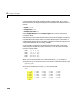
The computational delay of a block or subsystem is related to the number of
operations involved in executing that component. For example, an FFT block
operating on a 256-sample input requires Simulink to perform a certain
number of multiplications for each input frame. The actual amount of time that
these operations consume (as measured in a benchmark test, for example)
depends heavily on the performance of both the computer hardware and
underlying software layers, such as MATLAB and the operating system.
Computational delay for a particular model therefore typically varies from one
computer platform to another.
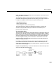
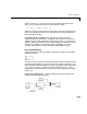
The simulation time represented on a model’s status bar (which can be
accessed via Simulink’s Digital Clock block) does not provide any information
about computational delay. For example, according to the Simulink timer, the
FFT mentioned above executes instantaneously, with no delay whatsoever. An
input to the FFT block at simulation time t=25.0 is processed and output at
time t=25.0, regardless of the number of operations performed by the FFT
algorithm. The Simulink timer reflects only algorithmic delay (described
below), not computational delay.
The next section discussed methods of reducing computational delay.
Reducing Computational Delay
There are a number of ways to reduce computational delay without actually
running the simulation on faster hardware. To begin with, you should
familiarize yourself with “Improving Simulation Performance and Accuracy” in
the Simulink documentation, which describes some basic strategies. The
section below supplements that information with several additional options for
improving performance.