User`s guide

Filters
4-7
where y(k) and u(k) are, respectively, the output and input at the current time
step, y(k-1) and u(k-1) are the output and input at the previous time step, and
so on. The values b
1
, b
2
, ..., b
m
, and a
2
, ..., a
n
are the filter coefficients, or taps.
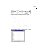
Every realizable filter is therefore fundamentally a collection of
multiplications, additions, and delays. The order in which these assorted
operations are implemented in practice determines the filter structure (also
known as the filter realization, architecture, or implementation).
Implementations may differ from each other in terms of speed, memory
requirements, delay, and quantization error. See “Linear System Models” in
the Signal Processing Toolbox documentation for more information about
common filter structures.
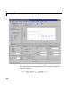
The Filter Designs library provides a number of blocks for designing filters
with various filter structures:
•Digital Filter Design
•Filter Realization Wizard
•Overlap-Add FFT Filter
•Overlap-Save FFT Filter
•Time-Varying Direct-Form II Transpose Filter
•Time-Varying Lattice Filter
See the following demos, which make use of many of the filter structure blocks:
•Frequency Domain Filtering (
olapfilt)
•LPC Analysis and Synthesis of Speech (
dsplpc)
•Sample Rate Conversion (
dspsrcnv)
Open the demos by clicking on the demo names above in the MATLAB Help
browser. Alternatively, open the demos by typing the demo name (provided in
parentheses above) at the MATLAB command line.
Designing Continuous-Time Classical IIR Filters
The Analog Filter Design block designs and implements continuous-time IIR
filters with standard band configurations. All of the analog filter designs let