User Manual

CUEMIX FX
93
A/B (stereo audio channels)
The View section (Figure 9-49) displays the pair of
input or output audio channels you are viewing.
See “Choosing a channel pair to display” above.
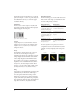
Line/Scatter
Choose either Line or Scatter from the menu in the
View section (Figure 9-49) to plot each data point
as either a single pixel or as a continuous line that
connects each frequency data point to the next, as
shown below in Figure 9-44.
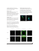
Figure 9-50: The same Phase Analysis displayed in Line versus Scatter
mode.
☛ Line mode is significantly more CPU intensive
than Scatter. You can reduce Line mode CPU
overhead for the Phase Analysis display by
increasing the Floor filter and reducing the Max
Delta Theta filters (see “Filters” on page 94).
Color/Grayscale
In Color mode (Figure 9-49) signal amplitude is
indicated by color as follows: red is loud and blue is
soft. In grayscale mode, white is loud and gray is
soft.
Linear/Logarithmic
Choose either Linear or Logarithmic from the
menu in the View section (Figure 9-49) to change
the scale of the frequency axis. In rectangular
coordinates, the vertical axis represents frequency,
and in polar coordinates, the radius from the
center is frequency. With a linear scale, frequencies
are spaced evenly; in a logarithmic scale, each
octave is spaced evenly (frequencies are scaled
logarithmically within each octave).
Linear is better for viewing high frequencies;
logarithmic is better for viewing low frequencies.
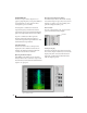
Rectangular/Polar
Choose either Rectangular or Polar from the menu
in the View section (Figure 9-49) to control how
audio is plotted on the Phase Analysis grid.
Rectangular plots the audio on an X-Y grid, with
frequency along the vertical axis and phase
difference on the horizontal axis. Polar plots the
data on a polar grid with zero Hertz at its center.
The length of the radius (distance from the center)
represents frequency, and the angle (theta)
measured from the +y (vertical) axis represents the
phase difference in degrees.
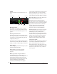
Figure 9-51: Rectangular versus Polar display (with a linear plot).
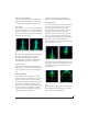
Above, Figure 9-51 shows Rectangular versus Polar
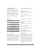
display with a Linear plot. Below, Figure 9-52 show
s the same displays (and the same data) with a
Logarithmic plot:
Figure 9-52: Rectangular versus Polar display with a logarithmic plot.
Axes
The Axes control (Figure 9-49) sets the opacity of
the grid displayed in the graph, from 100% (fully
visible) down to 0% (fully hidden).