User manual

Chapter 6 State-Space Design
Xmath Control Design Module 6-18 ni.com
numerical difficulties are encountered, the algorithm will attempt
to determine whether or not the problem is well posed. Checks are
made to determine the reachability and the positive definiteness or
semipositive-definiteness of the covariance matrices.
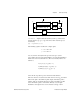
Because not all the values in the state vector are directly available from
measurements, your goal is to find an estimate of the state vector which
minimizes, in a least-squares sense, the error between the actual state vector
and the estimated state vector. This estimated vector is denoted by
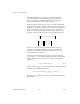
Because you want to minimize the error between this estimate and the
actual state values, the quadratic expression to be minimized becomes:
For the case of a discrete-time system, this quadratic expression is
evaluated as a summation rather than as an integral. No additional
information is provided by the inclusion of the Du term, so it can be
omitted without loss of generality.
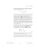
A derivation of the differential equation for the continuous-time state
vector estimate, can be found in [Kai81]. In the limit, this differential
equation, which provides the values for the continuous-time optimal
estimator, is
(6-5)
where K
e
=(PC'+Q
xy
')Q
yy
–1
and where the matrix P is obtained by solving
the algebraic Riccati differential equation:
The two preceding equations describe the continuous-time Kalman-Bucy
filter [KaB61].
x
ˆ
.
J
xt() x
ˆ
t()–()′yt() y
ˆ
t()–()′
•
0
∫
=
Q
xx
Q
xy
Q
xy′
Q
yy
xt() x
ˆ
t()–()
yt() y
ˆ
t()–()
dt
x
ˆ
,
x
ˆ
·
AK
e
C–()x
ˆ
Bu K
e
y++=
0 PA' AP PC' Q
xy
+()Q
yy
1–
Q
xy'
CP+()– Q
xx
++=