User manual

Chapter 1 Introduction

You can use the default exponential discretization method with dt =0.01

and compare frequency responses between the original system and the

discretized system:

ssysd = discretize(ssys, 0.01);

f = freq(ssys,logspace(.001,10,200));

fd = freq(ssysd,logspace(.001,10,200));

In the following statements you compute the gain and phase of both

systems and then plot them.

db = 20*log10(abs(f)); ph = (180/pi)*atan2(f);

dbd = 20*log10(abs(fd)); phd = (180/pi)*atan2(fd);

plot([db;ph;dbd;phd],{strip=2,xlog,

ylab = ["Gain (dB)";"Phase (deg)"],

x_lab = "Frequency (Hz)",

legend = ["ssys";"ssysd"]})

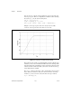
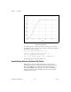
In Figure 1-11 you can see the frequency responses match closely,

indicating that this discretization method captures the continuous system’s

dynamics accurately.

Figure 1-11. Frequency Response of ssys and Its Discrete Equivalent ssysd