User manual

Chapter 4 System Analysis

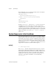
and orders for which the residue(s) should be found. If a user-specified

value for

pls is not actually a pole of the system or if the order requested

is greater than the multiplicity of the pole, the corresponding residue is

returned as zero.

C contains the value of the constant term.

Example 4-4 uses the transfer function from Example 2-10, Verifying a

Discretization Using makecontinuous( ).

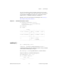
Example 4-4 Calculating the Residues of a System

G= system(0.5*polynomial([-0.36]),

polynomial([-1,-1,-0.395+0.06305*jay,

-0.395-0.06305*jay]));

Rp=residue(G)

Rp (a pdm) =

Poles |

-------------------+-----------------------------

-0.395 - 0.06305 j | Order 1 0.738493 - 0.2277 j

| 2 0

-------------------+-----------------------------

-0.395 + 0.06305 j | Order 1 0.738493 + 0.2277 j

| 2 0

-------------------+-----------------------------

-1 | Order 1 -1.47699

| 2 -0.864864

-------------------+-----------------------------

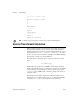
combinepf( )

Sys = combinepf(Rp,C,{var})

combinepf( )

reverses the operation performed by residue( ),

combining partial fractions into a single transfer function. It expects a PDM

of the form shown in Example 4-4 as input.

Use

combinepf( ) to convert partial fractions to a transfer function.

Using the variable

Rp you obtained in Example 4-4:

G2=combinepf(Rp, {var = "s"})

G2 (a transfer function) =

0.5s + 0.18

---------------------------

2 2