User manual

Chapter 4 System Analysis
Xmath Control Design Module 4-14 ni.com
Note A continuous system and its discrete-time equivalent (computed using the
impulse-invariant z-transform) have impulse responses differing only by a factor of 1/dt.
impulse( ) computes the impulse response by using the B matrix from
the system’s state-space representation as the initial conditions. A system
with n
i
inputs has n
i
initial conditions, each of which is set up as a column
of the B matrix. The impulse response is then a time-domain simulation of
the system using an appropriately-sized zero input.
The output
y is a PDM where domain is the time vector t. Each dependent
matrix in
y has as many rows as there are outputs of Sys, and as many
columns as there are inputs of
Sys. Thus the ( i,j,k ) element of y is the
impulse response at output
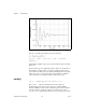
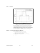
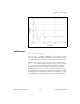
i from input j at time k. In Figure 4-4, where
all the poles of this continuous system are stable (in the left half of the
complex plane), the impulse response eventually dies out to zero. For an
example of a 15-second impulse response of a stable state-space system,
refer to Example 4-7.
Example 4-7 15-second Impulse Response of a Stable State-Space System
Sys = system([-2.3,0.01,5.1;0,-0.35,-2;0,2,-.35],
[1,.25,.25]',[1.34,0,0],0);
Yt = impulse(Sys,0:0.1:15);
plot (Yt, {xlab = "Time (sec)",
ylab = "Amplitude"})