
User`s guide

E-Prime User’s Guide
Chapter 3: Critical Timing
Page 97
3.4.1 Step 1. Test and tune the experimental computer
for research timing
Desktop computers come in thousands of hardware and software configurations. Most of these
can be tuned to provide millisecond precision as defined in section 3.2. However, there is a
serious risk that the current configuration of the computer cannot support millisecond precision.
Software programs may produce errors if they are running and taking up processor time during
the experiment. Also, there may be features/bugs in the hardware or driver software that distort
the timing. For example, some manufacturers of video cards do not reliably provide the
requested refresh rate, or provide the wrong signals. Compatibility testing early on in E-Prime’s
initial development cycle uncovered several cards that did not provide a vertical blanking
frequency, one card that provided the wrong frequency (the horizontal and vertical signals were
wired incorrectly), and cards providing the vertical blanking signal so briefly that most of the
vertical blanking events were missed. There are many good video cards available that can
provide good timing, and the system can be tuned for providing the demanding specifications of
millisecond timing.
Do not assume that your computer can provide millisecond timing. Test your computer
periodically and after every major hardware or software upgrade to verify that it can
support millisecond timing.
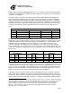
E-Prime offers testing programs to verify whether a machine can support millisecond precision
(see Appendix A, this volume). It only takes a few minutes to set up a test of your system. The
test can run short, one-minute tests, or long, overnight tests to assess the stability of a machine.
In addition, options can be set in E-Prime to log timing data along with behavioral data while
experiments are running. The timing test experiments will expose timing problems if they exist
and you are encouraged to use these tools to determine how different configurations produce
timing errors.
3.4.2 Step 2. Select and implement a paradigm timing
model
In the previous sections, the conceptualization of critical timing was covered. We will now begin
to address the specifics of how to implement paradigms with different timing constraints using E-
Prime and the tools it affords the researcher. However, before we review any specific paradigm
models we will begin with a few background discussions relating to identifying the true critical
timing needs of a paradigm, recommendations on specifying stimulus presentation times in E-
Prime applicable to most paradigm models, and timing issues associated with the overhead of
sampling stimuli and logging data within E-Prime.
The specific constraints of each individual paradigm dictate the necessary level of timing
accuracy and precision required. For the purposes of the following discussion, we will define
timing accuracy to be in one of two categories: critical and non-critical timing of events. Critical
timing is the situation in which there is a need to account for all events with millisecond accuracy
and precision. For example, the time between a stimulus and a mask typically requires critical
timing. Non-critical timing is the situation in which although the timing of events is recorded,
delays of a tenth of a second are not viewed as serious. For example, the onset and duration of
subject feedback or duration of the inter-trial interval in many experiments is non-critical at the
millisecond level. Therefore, a tenth of a second variation is generally of no consequence
experimentally. E-Prime affords users the ability to critically time all events over the course of
their experiments. However, doing so would require carefully specifying explicit durations,
PreRelease times and logging of every event. This would require a significant amount of time to
check the time logs of all the events to verify that the specifications were met. This amount of