MALÅ CX System Operating Manual v. 2.
Table of Contents _________________________________________________ 1 Introduction 3 1.1 Unpacking and Inspection 4 1.2 Repacking and Shipping 4 1.3 MALÅ Geoscience Indemnity Clause 4 1.4 Important information regarding the use of this MALÅ GPR unit 4 2 CX Start up 5 3 2D Project 12 4 3D Project 14 4.1 Creating a 3D Project 15 4.2 Migration settings and Images for 3D Projects 19 5 Object-Mapper Project 21 6 EM Option 23 6.1 Resulting signals/images 24 6.
1 Introduction __________________________________________________ Thank you for purchasing the MALÅ CX, the main unit for operating the MALÅ High Frequency antennas, both with and without EM option. CX10 gives you a High Brightness type of screen, while CX11 is equipped with a Trans-reflective screen for best performance in bright daylight. The MALÅ CX has built-in software for both data collection and on-site interpretation, tailored for high-frequency applications, as concrete investigations.
1.1 Unpacking and Inspection Great care should be taken when unpacking the equipment. Be sure to check the contents against those shown on the packing list and inspect the equipment for any loose parts or other damage. All packing material should be preserved in the event of damage occurring during shipping. Any claims for shipping damage should be filed with the carrier. Any claims for missing equipment or parts should be filed with MALÅ Geoscience. 1.
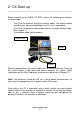
2 CX Start up __________________________________________________ Before starting up the MALÅ CX GPR system the following connections must be made: - - The CX to the antenna, using the antenna cable. The antenna cable should always be connected before the CX unit is powered on. The CX to the battery or other power source, using the battery cable. See Chapter 11. The encoder wheel to the antenna. Antenna cable Power Encoder When all connections have been made, the CX can be turned on.
There is also possible for the operator to navigate and execute all functions using the remote buttons on the antenna (Figure 12.5), the HF cart (Figure 12.2) and on the extension pole (Figure 12.6). By pressing either the black or red button the operator moves in-between the individual menus on the screen and activates the selection by pressing the two buttons at the same time.
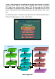
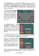
As seen three different measurement modes are available for the CX system; 2D, 3D and Object-Mapper Projects. All these project types are explained in detail in the following chapters. However, for all of these three options, general measurements settings are done first of all and in quite a similar way, so when selecting one of the options (2D, 3D or Object-Mapper) the following screen is seen, the General Settings window: www.malags.
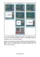
In this menu the options for changing Antenna, Material Type, Depth Window, Zero Depth, Acquisition mode (Wheel / Time) and Point Interval are found. If the Filters options in turned ON (done in the System Settings, see Chapter 9) it also shows up here. The trace and radargram view (right side of the screen) shows directly how the signal looks like. Moving the antenna over a surface will change this view of the wiggle trace and the gray scale background.
The Depth window (seen at right) defines depth of the measurement; in other words the total length of time the electromagnetic wave is transmitted. Three predefined depths are available, shallow, medium and deep. Choose the appropriate one by pressing the turn-and-push knob or use the remote buttons. Note! The depth window is depending on the velocity of the material. The option Find zero depth is used to define the surface level of the measurements.
After selection of material type or by choosing User-defined the option Velocity Wizard can also be entered to obtain correct velocity for the media. The requirement to use the Velocity Wizard (both for the migration and hyperbola fitting function) is that a point object needs to be visible in the radargram. Note! When using a hyperbola the best estimation of the velocity is made when the linear object is passed in 90 degrees.
Note! If you select a velocity value outside selected materials range, the material will be set to “User-Defined” The option Acquisition mode (in the General Setting view) and Wheel is changed depending on how the measurements are to be gathered; by time or by distance. If distance is chosen the correct encoder is selected. The standard MALÅ Geoscience wheels are found in the list. Point interval (or time in seconds) gives the distance between the measured traces in the radargram.
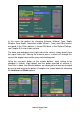
3 2D Project __________________________________________________ 2D Projects are defined as measurement in single profiles as seen below: Re-bars Concrete bottom This type of project can for instance be used to the investigate layer thicknesses, as concrete floors, asphalt thicknesses on roads, ice thickness etc. When the measurement settings (in the General Settings window) are done and is pressed the following screen is seen: 3 2 1 4 1: 2: Radargram screen (the resulting picture) Main menus. www.
3: 4: Battery Status Indicator Information Line showing the material type, the connected antenna type, measurement depth, memory space and acquisition mode. By choosing Start pressing the turn-push button, a radar profile measurement can be started immediately. By pressing the operator has the possibility to save a screenshot image of the radargram seen on the screen. Note! See Chapter 7 for measurements with a GPS. As each profile is completed, press STOP to finish the project.
4 3D Project __________________________________________________ 3D Project is a tool that makes the gathering and visualization of radar data measured in two perpendicular directions easier, directly in the CX unit. A typical application for which 3D Projects are effective is the mapping of rebars and joists in concrete. The 3D Project option in the CX will guide you through all steps involved in the data collection to the final processed 2.5D view of the investigated area.
some test measurements prior the 3D Project. This can be done by 2-3 single parallel profiles giving an indication of how the objects are situated. See Fig. 3.2. ma ir d- t G Figure 3.2 Three single profiles are measured, and indications of objects are marked with red. The 3D Project is carried out with one direction along the interesting objects and one direction perpendicular to the objects. 4.
line spacing, the grid size will also change to become the nearest divisible value. The same applies the values of Grid size. Press continue to reach the 3D Grid project layout screen to do a final check of the project parameters: Choosing Start activates the 3D Project. During data collection the two buttons on the antenna or on the extension handle are used as remote controls, for choosing the Next profile and Start profile. The number in the blue rectangle refers to the distance on the grid carpet.
4) Press the red button (to change measurement line), and wait for a beep. 5) Place the antenna in the start position of the next line and start from step 1 again. If black button is pressed after a profile is collected, the software assumes that the operator want to re-measure the current profile. The option can also be chosen to re-measure the previous lines. When all lines in one direction are measured, the CX system automatically will change to the second direction.
For explanation of the three function buttons: section in this manual. see next The options Angle, Aperture and Threshold are filter settings for the Top View and stands for: Angle – The space between the single lines of data is being filled with the help of an interpolation scheme. This interpolation can be performed in different directions the angle parameter determines this direction, -45 – +45. A value of 0 indicates orthogonal interpolation, the normal case.
Full-screen Saved screenshot The measured projects and created images can of course also be uploaded to a computer (see the section on Transferring Data). 4.2 Migration settings and Images for 3D Projects When the 3D project is ready, there are a number of different options available on the screen, in addition to the filter settings explained above. By pressing , the user can view the settings of the project. www.malags.
By pressing the button, it is possible to change the Velocity settings (Migration) or to create Image Slices. Note! Make sure that a welldefined hyperbola is visible in the right hand screen before entering the Velocity Settings (Migration window). Migration is a processing scheme which can significantly sharpen the radar image, especially when seen in the top view. Using this option, an appropriate velocity for the migration can be selected, by changing .
5 Object-Mapper Project __________________________________________________ An Object-Mapper Project is a tool to easily handle and interpret radar profiles acquired with the MALÅ CX system, where a number of radar profiles are measured parallel starting from a common baseline. See the example below. Applications can be for instance; mapping pipes, conduits or other larger linear structures, over larger areas.
Give the distance between the profiles, decide direction and line spacing. The direction right and left is defined as shown below: 2nd 1st 1st 2nd Profiles are made on the right-hand st side of the 1 profile Profiles are made on the left-hand st side of the 1 profile Note! In an Object-Mapper project the measurement lines are measured parallel to each other and orthogonal to the baseline.
6 EM Option _______________________________________________________ The MALÅ High Frequency antennas are also available with an EM option. These antennas are equipped with 50/60Hz electromagnetic (EM) sensors, to provide the CX with a combination of the radar and EM technologies to better locate and identify energized power cables, rebar, post-tension cables plus metallic and non-metallic conduits in concrete slabs either suspended or on grade.
The EM option is of course also active when measuring 3D Projects. The results of the EM measurements can be displayed as a Top view, on the 3D Project 2,5D View screen when selecting the option EM Data. The EM-option is mainly designed for detection of the leakage from AC power lines. This leakage is highly dependent on how the cable is designed i.e. a cylindrical twisted cable will have much less leakage than the cables commonly put into plastic pipes in walls.
be different. For other cable geometries there may be only one peak over the cable. When the cable is twisted the EM signal can vary very rapidly over short distances, making precise location of the cable more difficult. In the 3D Project view the average signal at each point of measurement is plotted along each survey line and then interpolated over the surface. The location of any cable will be highlighted by areas of larger EM variation.
7 GPS Functionality __________________________________________________ The CX system is available with a positioning system, GPS, which can be used with 2D and Object Mapper measurements. To activate this functionality an activation code is needed (contact your local sales representative for more information). The GPS is connected to the CX main unit via the USB port. When a GPS is connected the system immediately start to log the positioning data with x, y and z-coordinates.
The MALÅ GPS standard, GPS format contains the following information: trace number, date, latitude, longitude, height above mean sea level, and HDOP. The HDOP value is a theoretical measure of the accuracy in the horizontal coordinates based on the positions of the available GPS satellites. A lower value indicates better accuracy. The date and time is expressed in Greenwich Time zone.
8 File Manager __________________________________________________ As a profile measurement is started (2D Project) the data is automatically saved and named as in the following files: - 2D_0001.rd3 - data (traces) 2D _0001.rad - header (measurement info) 2D_0001.cor – coordinates if a GPS I connected to the system 2D _0001.em - EM data (if using antennas with EM option) During a 3D Project the following data file is created: - - 3D_0001.
Every file belonging to a specific measurement has the same file name, and the file extension specifies the type of data in the file. The previously measured files can be viewed within the CX by pressing Work with Files in the main menu. Under this menu, the operator can choose to view files, delete them or upload those (See Section Transferring Data). To select a file turn the turnpush button to the file name and press to select. To mark and select several files at the same time, use the Mark option.
8.1 Transferring data By connecting a flashcard (USB storage media) to the USB port at the top left corner of the CX the measured data can be easily transferred by pressing in the File dialog (See the section File Manager). All marked files and grid projects will then be copied to the storage medium, which can then be connected to any desired computer. The USB port is found top left, under the black cap. www.malags.
9 System settings __________________________________________________ The System menu of the CX unit can be reached after choosing Quit on the main menu, as if to shut down the unit. It is reached by turning the turn-push button 3 clicks right, 3 clicks left and 3 clicks right at the following screen. In the System Menu the following changes are possible: - Time and date - Battery installation to set battery indicator level - Activate the kill-switch. See below. - Missed traces.
- - Software upgrade. See Chapter 10. Restoration of predefined settings. See Below. Restoration factory Settings. See below. Note! By pressing reached. the next System settings screen is By activating the kill-switch (mandatory under certain conditions, due to FCC regulations, see FCC Part 15.
activate the kill-switch). The use of a kill switch function makes the antenna stop emitting electro-magnetic waves when the switch is released. Note that it’s advisable to continue with the next line within 10 seconds to avoid any time drifts of the signal. The CX system will work in the following manner: - - By default the Kill-switch is always OFF and transmitting is always enabled.
Here it is possible to change the parameters for the two different CX filters, the FIR filter and the Time Gain filter. If one of the buttons are pressed then the Trace/Radagram View will show how the choice of filter parameters affects the trace otherwise the Trace/Radagram View will show the trace/radargram only with DC removal filter. If the FIR switch is OFF then DC Removal filter is ON for all displayed data.
Pressing Restore Predefined Settings the system file in the CX restores the following: - All antennas and wheel parameters will be restored - Battery level is set to 11 V - Meters are chosen as the measurement units By pressing Restore Factory Settings the system file in the CX is restored from the system file default image. This is useful if the system file in the unit has been damaged in some way.
10 Upgrade __________________________________________________ The instructions below describe how to upgrade the application software of the CX. 1. Download the file: “ECX_080021.zip”. The file must be unzipped once and then a file named “ram10img.gz” is seen, which is zipped as well, but should remain so. 2. Copy the file “ram10img.gz” to a USB flash memory. 3. Connect the unit to a fully charged 12V power source and start it up.
11 Batteries and Power supply __________________________________________________ Note! Before use, open the battery pack and connect the battery to the outside connectors. See figure below. The Li-Ion battery pack is the standard power supply for the CX main unit. The capacity of the battery is 12V/13.2 Ah. This gives an operation time of approx. 6 hours depending on the settings and configuration of the system. The battery should always be stored fully charged to maximize the lifetime of the battery.
12 High Frequency antennas ___________________________________________________________ MALÅ High Frequency (HF) antennas are available with frequencies of 1.2, 1.6 and 2.3 GHz. The 1.2 and 1.6 GHz antennas also have an EM (Electromagnetic) option, giving a GPR antenna with a 50/60 Hz EMlocator. The HF antennas are most suitable for investigations were high resolution is important, as for construction/concrete investigation, asphalt mapping, ice thickness etc. See also Table 12.1. Table 12.1.
Figure 12.2 The HF antenna (1.6 or 2.3 GHz) in a wheel carriage, the HF cart. Note the connections for the encoder wheel and the antenna buttons. Figure 12.3 Mounting the HF antenna in the HF cart. The antenna is attached to the cart on two sides, see the arrows. The HF antennas are attached to the CX main unit through a 4 m long cable, allowing a flexible and mobile data collection. A 10 m extension cable is also available.
used in another measurement direction, for instance to investigate polarization effects. Figure 12.4 The single wheel encoder (top) and attached to a HF antenna (below) in two different directions. When the HF antennas are used with the CX control unit, the data collection can also be controlled by the two buttons on the handle of the antenna (Fig. 12.5), or on the HF cart or extension pole.
Figure 12.6 Extension pole. On the handgrip the two buttons are seen, the one on the top (red) starts a new profile. When using the extension pole, as seen in Fig. 12.6 above, the two buttons are located on the hand grip, with one button underneath the grip starting and stopping the data collection, and the other one (red) on the handle top starting a new profile.
As an option a switch box is provided to the High Frequency antennas (Fig. 12.8). With this switch box it is possible to measure with only the receiver in one HF antenna and only the transmitter in the other HF antenna. This enables different types of tomographic measurements and velocity analysis as CMP (Common Mid Point). The data cables from the two antennas are connected to the switch box and the switch box to the CX Main unit. Figure 12.8. Switch box for two High Frequency antennas. www.malags.
13 Technical Specifications CX unit __________________________________________________ Pulse repetition frequency Data bits Time stability Sampling frequency Acquisition mode Time Window Power supply Operating time Charger Charge time Input device On/Off Screen Antenna compatibility Dimension Weight Operating temperature Environmental Data download Data memory 100 kHz 16 Better or equal than 60 ps 6-700 GHz Distance/time/manual, Grid measurements are controlled by remote controls on antenna/handle, w
14 Technical specifications HF Antennas __________________________________________________ Centre frequency 1.2, 1.6 and 2.3 GHZ Bandwidth > 100 % Time window > 50 ns Repetition rate 100 kHz EM option 50 Hz or 50/60 Hz sensors (sensitivity 300 uV, 14 bits) Dimension 160x90x110 mm (1.6 GHz and 2.3 GHz) and 190x115x110 mm (1.2 GHz, 1.6+EM and 1.2+EM) Weight 0.6 kg: 1.6 GHz and 2.3 GHz 1.0 kg: 1.2 GHz 1.2 kg: 1.6+EM and 1.
www.malags.com Corporate Headquarters Offices MALÅ Geoscience AB Skolgatan 11, SE-930 70 Malå, Sweden Phone: +46 953 345 50 Fax: +46 953 345 67 E-mail: sales@malags.com USA: MALÅ Geoscience USA, Inc., 465 Deanna Lane, Charleston, SC 29492 Phone: +1 843 852 5021, Fax: +1 843 284 0684, E-mail: sales.usa@malags.com China: MALÅ GeoScience (China), Room 2604, Yuan Chen Xin BLDG, No.12 Yu Min Road Chao Yang District, Beijing 100029 Phone: +86 108 225 0728, Fax: +86 108 225 0815, E-mail: sales@malags.