
Basic Documentation
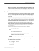
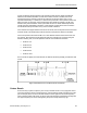
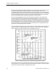
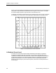
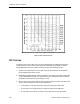
Table Of Contents
- About this Application Guide
- Chapter 1–Introduction
- Chapter 2–Physics of Sound
- Chapter 3–HVAC Sound Sources
- Chapter 4–HVAC Sound Attenuation
- Introduction to HVAC Sound Attenuation
- Plenums
- Duct Attenuation
- Duct Takeoffs and Divisions
- Duct Silencers
- End Reflection
- Environment Adjustment Factor
- Space Effect
- Radiated Sound Attenuation
- Chapter 5–HVAC System Sound Analysis
- Chapter 6–Minimizing HVAC Sound
- Appendix
- Glossary
- Index

Chapter 2–Physics of Sound
Previously, we discussed the terms sound power level and sound pressure level and arrived
at how their intensity was expressed in decibels. If you recall how the screen of an
oscilloscope looks when it’s monitoring the audio output of a speaker, you can visualize that
sounds are usually composed of a multitude of tones at different frequencies. To scientifically
describe a particular sound accurately, a curve should be plotted showing the sound power
level or sound pressure level in decibels with reference to the frequency.
Since the normal audible spectrum covers the frequency range of 20 Hz to 20,000 Hz, it
would be totally impractical to deal with each individual frequency. For this reason, it has
become customary in sound analysis to divide the overall audible spectrum into 8 frequency
bands called octave bands. (These are often referred to as 1/1 Octave Bands.) In each band
the highest frequency is twice the lowest frequency, and the mid frequency of each band is
used for identifying the octave band and as the specific frequency for expressing the sound
power level or sound pressure level in decibels.
Figure 3 illustrates how sound curves can be shown on a graph that plots the sound pressure
level at each of the standard octave band mid frequencies. The resulting curves establish
what’s referred to as a sound criterion curve for the particular sound.
Figure 3. Sound Pressure Level vs. Octave Band - Sound Criterion Curves.
With reference to Figure 3, the dB scale ascends from 0 to 90 along the vertical axis and the
center frequencies of 10 bands are along the horizontal axis. Note that the frequency scale is
not linear but increases rapidly in moving from left to right.
14 Siemens Building Technologies, Inc.