WIYN High-Resolution Infrared Camera (WHIRC) Quick Guide to Data Reduction Dick Joyce Version 2.0, 2014 June 26 WHIRC Data Reduction Manual Version 2.
ACRONYMS AND ABBREVIATIONS: ............................................................................................................. 2 1.0 INTRODUCTION............................................................................................................................... 3 2.0 DATA PREPARATION ..................................................................................................................... 3 2.1 2.2 2.3 2.4 2.4.1 2.4.2 2.4.3 2.4.4 3.0 DATA REDUCTION .....................
WIYN High-Resolution Infrared Camera (WHIRC) Data Reduction Guide 1.0 Introduction This document is a quick guide to reducing data taken with the WIYN High Resolution Infrared Camera (WHIRC). Data reduction is a highly personal process, so one should keep in mind the procedures described here are biased by the author’s personal preferences and experience. Many WHIRC users may have their own (possibly superior) means of reducing data, or use reduction platforms other than IRAF.
obtained within a fairly narrow time window. We strongly suggest that observers who generate sky flats also obtain dome flats as a backup. 2. Science Observations: These can be a series of dithered observations on the source field (for standards and pointlike sources) or a set of dithered observations on the source and a set of dithered observations at an off-source sky location. 3.
2. Scaling: If any of the data were taken with Fowler-4 mode, the pixel values must be normalized by a factor of 4 prior to any linearity correction. The Fowler-4 mode adds all of the four readouts but does not divide by 4 to avoid possible noise digitization in the integer output format. So for the Fowler-4 data only: imarith *.tr.fits / 4. *.tr.fits will do this in place.
correctly displayed on the image display. ROTOFF is normally 0.0, but at some telescope orientations, the WIYN instrument rotator has to rotate by 180 degrees because of the limited cable loop. Also, observers may intentionally rotate the instrument to a non-cardinal orientation to fit an elongated target onto the array. These offsets are properly recorded in the ROTOFF keyword, but not in the raw image display at the telescope. After executing wprep.
2.2 Generating Dome Flats It is generally a good idea to run imstat on the flats just to identify any possible bad frames and eliminate them from the input data. 1. For each of the on/off sets in the filters, imcombine each set into a single image (e.g., flat.k.on, etc.). One can generally use ‘combine’ = average, with avsigclip rejection, although median should work as well.
Figure 2.3: IRAF parameter listing for the imcombine task to combine flatfield images (in the list ‘flatlist’) into a combined ‘on’ flat. For the ‘off’ flat images, we recommend setting ‘scale’ = ‘none’, since the signal levels are generally small. WHIRC Data Reduction Manual Version 2.
Figure 2.4: Normalized flat for Ks (left panel) and J (right panel). The significant difference in the two emphasizes the need to obtain dedicated flats in each filter used for observing. The pupil ghost in the J band is much less prominent, but there is a noticeable “fingerprint” artifact, probably resulting from a defect in the antireflection coating on the array. Note that the bad column has been set to a value of 1.0 by imreplace. Figure 2.
1. Sky flats are best generated from a series of observations which give an appreciable (several thousand ADU) sky level. This pretty much restricts nighttime observations to the H and Ks filters. Twilight flats can be taken in the J and (perhaps) narrowband filters, but the rapid onset of twilight in the infrared leaves limited time for this procedure. H band sky flats may show fringing from the OH lines, which will complicate the process (section 2.4.4). 2.
2.6, 2.7). The smooth variation evident in a cut through one of the dimples (Fig. 2.7) would make pixel correction algorithms (such as ‘fixpix’) based on nearest neighbor averaging problematic. Figure 2.6: Expanded subregion of H band image, showing some of the “dimples” on the detector (left panel). These are not dead pixels and appear to divide out using a flatfield (right panel) to within 1 – 2 %. Figure 2.
and use imreplace to set the pixels deviating from what should be a narrow distribution to the “bad pixel value” in the image. Typically bad pixel maps utilize a value of 1 for bad pixels and 0 for good pixels (Fig. 2.8). Figure 2.8: Bad pixel image bpix.whirc.fits generated from the ratio of two dome flats. In addition, one can generate a bad pixel file (which typically has a .pl extension) to identify specific pixels or regions which are bad.
2.4.1.4 Photo-emitting Defects Photo-emitting defects (PEDs) are generally pixels which become shorted during the hybridization process. They draw significant current during the bias reset and emit light. PEDs are generally identified during the testing stage by the vendor and “cauterized” using a laser. This produces a region of limited sensitivity approximately 20 pixels in diameter, surrounded by a bright annulus. The WHIRC detector has at least two PEDs, centered near [337:266] and [839:1804].
Using gauss with sigma=31 gave a similar result; observers may want to try both of these strategies. Figure 2.10 : IRAF parameter listing for the fmedian task, to smooth out the ratio of the Ks/J flats. The ratio had been previously edited with imreplace to knock down some of the bright spots in the ratio. Fig 2.11: (left panel) Ratio of reduced dome flats in Ks and J. Note that the bright region near [1250:1250] cancels out of the ratio, suggesting it is a response variation common to both wavelengths.
tapers to near zero at the edges. One can then copy the central 800 × 800 region into the zero image to get something like the image in Fig. 2.11b. You may need to play with the level of the zero image to get a smooth transition to the pupil subregion. Figure 2.12: IRAF parameter listing for the task mkimage. This will generate a 2048 × 2048 image ‘whircpupil.fits’ with pixel values of 0. Figure 2.13: IRAF parameter listing for the task rmpupil. WHIRC Data Reduction Manual Version 2.
Fig. 2.14: Dome flat for Ks before (left panel) and after (right panel) removal of bad pixels and the pupil ghost. Note the bright region near [1250:1250] remains. The pupil template can then be used with the task ‘mscred.rmpupil’ (Fig. 2.13) to remove the pupil ghost from the flat. A representative pupil template (whircpupil.fits) can be downloaded from the WHIRC webpage, although observers may wish to create their own. The pupil mask (pupmask.
4. Set pixels below a certain value (say 0.05) to 1.0 to avoid excessively large numbers in the flattened image using imreplace (Fig. 2.5). Alternatively, ensure that a bad pixel map includes low-valued pixels. 5. Copy flats to a “fixed” extension: imcopy flat.140420.*.fits flat.140420.*.%fits%fx.fits% and run fixpix on these images (Fig. 2.9). 6. Generate a rough image of the pupil ghost by dividing the processed Ks flat by the J flat: imar flat.140420.fx.k / flat.140420.fx.j flatrat.kj 7.
Because the strength of the OH lines varies during the night, fringes may not be seen in the sky frame (see section 3.1) for any given target, but they may very well appear in a “supersky” generated from all of the observations during a given night. This is often the case in the H band; in the Paβ and Paβ45 filters, the fringes will almost always be prominent since the continuum sky background is negligible and science exposures tend to be long. The MOSAIC reduction task mscred.
Figure 2.15: IRAF parameter list for the task imcombine to obtain a sky image for the set of images in the file ‘inlist’. Note the use of ‘combine’ = ‘median’ to remove the stars from the dithered images. This sky frame can be used for sky subtraction, generating a sky flat, or generating a fringe template. The process is similar for generating a dark image from a series of images, except the scale should be set to ‘none’ since the signal levels are very low. WHIRC Data Reduction Manual Version 2.
Figure 2.16: Average of sky images in the Paβ filter (left panel), showing evident fringes. Same image after subtraction of dark frame (right panel). 3. At this point most of the dark current will be removed, except for occasional mavericks, but the frame still has the low spatial frequency structure and the central pupil ghost. Dividing by the dome flat and running fixpix with the bad pixel mask (Fig. 2.9) will remove most of the structure and clean up the image (Fig. 2.18a). 4.
For comparison, we show in Fig. 2.19 fringe templates for the Paβ45 and H filters, to show the need for filter and time-specific fringe information. While the Paβ45 pattern seems similar to the Paβ pattern, one can see a phase difference in the central fringe. The fringe visibility in the H band varies, suggesting that several emission lines contribute to the fringes. Figure 2.18: (left panel) Paβ sky image from Fig. 2.16b after dividing by a dome flat and cleaning up bad pixels.
5. Using the appropriate fringe template, the task rmfringe can then be used to remove the fringes (Fig. 2.20). Figure 2.21 illustrates this for a H band sky image on a night where fringing was evident. In practice, one would operate on a sky-subtracted image, where the fringe pattern should be much less evident. Figure 2.20: IRAF parameter listing for the task rmfringe using the smoothed Paβ fringe pattern from Fig. 2.17b. Fig. 2.21: H band sky image (left panel) on a night when fringing was evident.
3.0 3.1 Data Reduction Standards or Pointlike Objects 1. One will generally have several images of the field with different telescope pointings. Depending on the sky stability, the sky level may be somewhat different in each of the images. 2. Create a sky image using imcombine on all of the images in a given filter on each target field with median filtering, as described in section 2.4.4.
5. One may analyze the results from each image separately or combine them, using upsqiid or other custom routines. 3.3 Combining Images into a Mosaic For IRAF users, the upsqiid package written by Mike Merrill can be used to align and combine the images into a single image. This is primarily useful for deep imaging, where one is observing the same field with relatively small dither amplitudes, since it relies on locating star(s) common to all images for alignment.
During the design of WHIRC, the entire optical system (WIYN telescope, WTTM, and WHIRC) was modeled using Zemax, and optical distortion maps were generated in the J, H, and Ks filters. These files were used as input to the IRAF routine geomap to generate third-order polynomial fits with an rms error ~ 0.1 pixel. The files whirc.distort..txt and whirc.distort..
Figure 3.1: Parameter file for the geotran task. 3.3.2 Small Field Mosaics The two basic tasks within the upsqiid package which are useful for combining images: xyget – Find common stars in the images and create a registration database nircombine – Combine the registration database into a composite image 3.3.2.1 The xyget Task The task xyget is an interactive task in which each of the images is displayed in turn and a star common to all of the images is identified on the display.
1. Reduce the images to be mosaicked (sky subtraction, flatfielding, etc.) as above and put them into a list. 2. I usually like to set the sky levels for all of the images to zero before running xyget, but this is optional, since one can also carry out this step automatically within the nircombine task. (Although the two approaches seem to give slightly different sky levels in the combined image). One needs to set the imstat task so that the mode (or midpoint) is one of the output columns: a.
Figure 3.2: Parameter set for the task xyget without distortion correction. The parameter ‘tran’ is set to ‘no’. WHIRC Data Reduction Manual Version 2.
Figure 3.3: Parameter set for the task xyget with distortion correction. The parameter ‘tran’ is set to ‘yes’. Figure 3.4: Output at completion of the xyget task. Note that all of the five images have offset data. WHIRC Data Reduction Manual Version 2.
3.3.2.2 Combining Images with nircombine The task nircombine (Figure 3.5) will combine the input images using the ‘.xycom’ output of xyget. Figure 3.5: Parameter set for the IRAF task ‘nircombine’. The ‘apply_z” parameter is set to ‘yes’ to normalize any offsets in the sky level of the input images. a. The first parameter ‘match_na’ will be the name of the resultant image WHIRC Data Reduction Manual Version 2.
b. The parameter ‘infofile’ is the ‘.xycom’ output file from xyget. c. The parameter ‘frame_n’ is the list of images one will combine. Normally, this would be the entire set of input images, but there may be reasons (bad seeing, telescope jump, etc.) why one may wish to exclude some images. d. The parameter ‘comb_op’ specifies the method used for combining the images.
filtering algorithm. (lower left) Difference of the top two images. Note that the sky subtraction reduces the residual background to near zero. (lower right) After flatfielding, the nine images are combined into a single composite using the upsqiid tasks xyget and nircombine. Note that the noise is higher in the periphery of the image where only a single image contributes to the mosaic.
nearby sparse field with a median filtering algorithm. (lower left) Difference of the top two images. Note that the sky subtraction reduces the residual background to near zero. (lower right) After flatfielding, the five images are combined into a single composite using the upsqiid tasks xyget and nircombine. Note that the noise is higher in the periphery of the image where only a single image contributes to the mosaic. This image is displayed using a logarithmic scaling to bring out faint details.
and that the data be taken in a regular N × M mosaic pattern. The process is a bit cumbersome in that one must manually generate and edit a file containing the relative coordinates of reference stars in adjacent images. The irmosaic task combines the input images into a single N × M mosaic, in the same geometry that they were taken on the sky. It is important that one inspect the mosaic image to ensure that the component images are in the right order. The apphot.
just to make the separation of the input images in the output mosaic obvious (Figure 3.10). It is easy to identify the common stars in the mosaic. Figure 3.10: Output image sak.j.mos.fits generated by the irmosaic task. One can now display the mosaic image and run the apphot.center task on it by centering the cursor on a star and hitting to measure the centroid. This must be done in pairs, measuring the same star in two adjacent subimages in the mosaic image.
Figure 3.11: Parameter file for the IRAF task irmatch2d. Figure 3.12: Aligned image resulting from the irmatch2d task. WHIRC Data Reduction Manual Version 2.
4.0 4.1 Appendices Appendix A – Observational Test of Pupil Ghost Removal On the (apparently) photometric night of 9 July 2009 UT we tested the pupil ghost removal technique described in section 2.4.2 by sampling a region approximately 80 arcsec square centered on the array.
The sky subtracted images were flattened with both the uncorrected and nopupil flats, yielding three datasets of 100 images each: • • • Sky-subtracted, unflattened images Uncorrected flattened images Pupil corrected flattened images The selected star was measured using apphot with a fairly large (4 arcsec diameter) aperture to minimize the effects of seeing or focus drifts for all three datasets.
Figure 4.1: Plots of the magnitude of a Ks ~ 11 star measured in a 4 arcsec aperture using the IRAF task apphot over a 10 × 10 raster centered on the WHIRC pupil ghost. The magnitude scale is not calibrated to a photometric standard. The same dataset is plotted for the sky-subtracted, unflattened data (top panel), data flattened with no correction for the pupil ghost (middle panel), and data flattened with correction for the pupil ghost (bottom panel). WHIRC Data Reduction Manual Version 2.
Figure 4.2: The pupil-corrected flattened data from the lower panel of Fig. 4.1, but plotted as a function of time, in the order the data were obtained. The line is a linear fit to the data and probably represents atmospheric extinction, since the airmass increased over the span of the observations by approximately 0.20. WHIRC Data Reduction Manual Version 2.