I-Track Real-Time Sound Mapping System & Automatic Sound Power Measurement User guide – V4.02 Soft dB Inc. 1040, Belvedere Avenue, Suite 215 Quebec (Quebec) Canada G1S 3G3 Toll free: 1-866-686-0993 (USA and Canada) E-mail: contact@softdb.
Contents 1 Introduction ............................................................................................................................. 1 2 Components ............................................................................................................................ 1 3 Warranty .................................................................................................................................. 2 4 Quick Start .......................................................
1 Introduction Congratulation on your purchase of the I-Track Sound Mapping System. I-Track is a powerful tool for easy and accurate sound intensity cartography. It combines machine vision with high performance DSP acquisition to produce sound intensity maps. The result is a low cost, accurate, easy to use tool appropriate for both field and laboratory measurements. Sound Intensity maps are the ultimate noise source analysis tool.
3 Warranty SOFT DB INC. warrants this instrument to be free of defects in parts and workmanship for one year from date of shipment (a six-month limited warranty applies on sensors and cables). Should it be necessary to return the instrument for service during or beyond the warranty period, please contact us at (418) 686-0993 for authorization or visit our website at www.softdb.com (Click on Contact for more information).
4 Quick Start 4.
Step 2 Take Background Picture Before performing a sound mapping measurement, a background picture must be taken. In order to do this, plug the digital camera on a USB port and click the “New Measure” button on the software interface or on the intensity probe: This will launch the background picture interface: This interface allows adjusting the camera parameters, such as focus, luminosity and contrast.
Step 3 Run a Measurement When returned form the background picture interface to the main interface, the recently acquired background image should be displayed in the map indicator. Click the “Run” button on the interface or press the equivalent button on the intensity probe to run the measurement. When the measurement starts, scan the virtual measurement plane. The sound map will be painted in real-time.
6
Step 4 Stop the Measurement When the measurement is done, click the “Stop” button on the software interface or press the corresponding button on the probe: If the “AutoSave” mode is enabled, the measurement is automatically saved in the record directory when the user stops the measurement: 7
Step 5 Post-processing When the measurement is recorded, the map computation process is launched. This computation process performs advanced operations on the acquired data to display a highly accurate result. These advanced functions require working on the whole dataset and therefore cannot be performed during the acquisition process. At any time the user can cancel this process to perform another measurement right away.
You can select the displayed band by clicking on the corresponding band on the spectrum. Step 6 Exporting Data The exported data consists of map images (.png) and spectrum data (Excel compatible .txt file). A simple image export can be performed by sending the current map to the clipboard and pasting it in the target document. Image sent to clipboard To export the current dataset, select “Export Current” in the “File” menu. This function will export all the maps as *.
5 Main Interface Menu Bar Nb Points Meas Indic. Map Scale Meas Ctrls Map Tools Comments Spectrum 5.1 File Ctrls Menu Bar The Menu bar allows access to different functions, interfaces and tools. • • • • File; • Open; • Save; • Save as; • Export current; • Export multiple; • Quit. Setup; • File setup (current); • Measure Setup (next); Tools • Field Check; • Field Indicators; • Playback; • Power-process; • 3D view.
• 5.2 • About; • Shortcuts; • User Guide. New Measure. Map Scale This area displays the color scale of the sound map and also displays the title of the dataset displayed in the map, such as global sound intensity or 1 kHz Sound Pressure. 5.3 • • • • 5.4 Map Tools Display setup: Access to the current display setup. Zoom map: Allows zooming the map. Copy map to clipboard: Copies the map image to the clipboard to paste in a target document.
5.7 Measure Controls These controls are used to control the measurement. These controls can be accessed either form the remote control probe or directly on the software interface. • • • 5.8 Run / Pause: Starts, pauses and resumes a measurement; Stop / Save: Stops and saves a measurement; New Measure: Launches the background picture interface. Comments These text controls allows the user to add comments to a measurement. • • 5.
6 Configuration Setup The configuration setup is an aggregate of different information which relates to a measurement such as: • • • File information; • Software version; • Start time-stamp; • Comment; • Etc. Input setup; • Microphone calibration; • Phase mismatch compensation; • Microphone spacer; • Etc. Etc. This information is recorded with the measurement file, dictates how the data is interpreted and provides useful information to the user when post-processing the files. 6.
6.2.2 Input This interface shows the inputs configuration. This is where the user can perform microphone calibration. Microphone A Microphone B Phase PI Residual Microphone Spacer Sensor Info The sensor info contains information such as manufacturer, model and serial number of microphones in use. It also allows defining the input channel, the range and the sensitivity of each microphone.
Amplitude Calibration The amplitude calibration interface allows calibrating the sensitivity of each microphone using a single-tone calibrator. To perform a calibration: 1) 2) 3) 4) Place the calibrator on the selected microphone and turn the signal ON; Set the appropriate frequency and amplitude of the calibration signal on the interface; Enter the calibrator info (optional); Click the “Start Calibration” button to launch the calibration process.
2) Insert both microphones in the calibration chamber; 3) Enter the calibrator info (optional); 4) Click the “Start Calibration” button to launch the calibration process. It is recommended to perform a phase mismatch compensation calibration before each measurement campaign. Some PI Residual calibrators require a certain time to equilibrate the pressure in the calibration chamber after the insertion of the microphones.
It is strongly recommended to perform an amplitude calibration and a phase mismatch compensation calibration prior to the measurement of the PI residual. Enabling phase mismatch compensation increases the PI residual and the dynamic capability of the instrument. Some PI Residual calibrators require a certain time to equilibrate the pressure in the calibration chamber after the insertion of the microphones.
Recommended frequency range for most common microphone spacers (mm) 6.2.3 Output This interface shows the output configuration. The outputs of the Conductor or the Alto can be used to generate different signals during the measurement. Two outputs can be used and several signal types can be combined.
6.2.4 Advanced The advanced parameters can be adjusted in this interface. Delta t The Delta t value sets the time interval between each acquired point. Therefore, the time signal equivalent for this measurement point will be averaged over this time interval. As an example, a 0,125 s time interval means that 8 points per seconds will be acquired and each of them will integrate the time signal on a 1/8 s duration. When FFT is selected, an overlap of 66.6% is applied as a result of the Hanning windowing.
Temperature, Pressure and Humidity The temperature, pressure and humidity parameters allow the user to define the atmospheric conditions prevailing during the measurement. The software will compensate the intensity results to provide standardised results at 20°C, 101.325kPa and 50% Humidity (ISO 5011). Grid Precision The grid precision defines de precision of the computing grid. Typically, the grid precision must be about 1/100 the source size to provide a good precision over computation speed ratio.
Pattern Size Microphone Offset Maximum Time and Maximum Speed The maximum time and speed refer to the tracking parameters. The maximum time specifies the maximum elapsed time between two acquired positions to validate the path between these two positions. Typically, 1 s maximum elapsed time is appropriate. The maximum speed specifies the maximum speed for a segment path to be valid. A maximum scanning speed of 0.5 m/s is required by ISO 9614-2.
6.2.5 Display The display interface allows setting several display parameters. These parameters are: • • • • • • • • • • • Spectrum: 1/1 Octave, 1/3 Octave or FFT; Weight: A, C or Z (no weight); Bandwidth: Low and high frequency range to consider.
Grid Points Tracks 6.2.6 Triangles Configuration File The configuration file allows saving all the settings in a single file to be recalled later or to transfer settings from an I-Track system to another. 6.3 Record Setup The Record Setup allows defining the record directory and the file prefix to use when auto-saving.