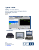
Opus Suite Building Acoustics Module Airborne Sound Isolation between Rooms ASTM E 336 / ISO 140-4 User Guide – v1.1 2012-12-06 Compatible Hardware: Alto 6-Channel Concerto 4-Channel I-Track 6-Channel Soft dB Inc. 1040, Belvedere Avenue, Suite 215 Quebec (Quebec) Canada G1S 3G3 Toll free: 1-866-686-0993 (USA and Canada) E-mail: contact@softdb.
CONTENTS 1 Introduction ........................................................................................................................... 2 2 Compatible Hardware ............................................................................................................. 3 3 Opus Environment .................................................................................................................. 4 4 Quick Start........................................................................
1 Introduction Congratulations on your purchase of the Opus Suite STC module. The Opus Software Suite is a Sound and Vibration software that contains several measurement modules: • • • • SLM 4-ch module : 4-channels, Class 1 (IEC 61672 and ANSI S1.
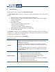
2 Compatible Hardware Every hardware option has an embedded state of the art Soft dB SR-MK3 DSP board allowing realtime and precise measurement with very low energy consumption. Concerto 4-Channel Alto 6-Channel I-Track 6-Channel Handy, lightweight, fully rugged military grade (MIL-STD-810F and IP67) tablet PC with anti-glare & anti-scratch touch screen All in one instrument (no PC required) WLAN communication allows using the Concerto as a monitoring station with remote access. www.softdb.
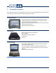
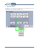
3 Opus Environment The Concerto unit comes equipped with the Opus Environment. This environment acts as a main interface that gives access to the different modules and tools.
Modules The modules buttons will launch the associated module. When a module is opened, a license verification check is done. If no license is found for that module, a message will indicate the limitations. The File Manger button will launch the File Manager Utility (see section 10, p. 26) The Software Install button will launch a browser from which an Opus software installer can be launched. The Network Manager button will launch the Network Manager interface.
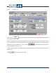
4 Quick Start The STC module is part of the Building Acoustic. It can be accessed in the Building Acoustic menu of the Opus Suite panel. Measurement tab Measure the selected element Elements to measure What you should know… • • • • • • The partition area and the receiving room volume are used to evaluate de STC.
Step 1 Setup the unit Click on the button to access the setup interface. The parameter should typically be set as shown on figure above. Before a measurement, the operator should set the sensitivity of the sensor used. This sensitivity can be set manually if it is known. Preferably, the sensor sensibility should be set by using the software calibration tool and a calibrator. To do so, click on Sensor Calibration (section 0, p.15).
Step 2 Do a Level Measurement Start the Average Accept the measurement To proceed to a measurement, select an element to measure in the table of the main panel and click the button to open the measurement interface. Once in the measurement panel, click on the button to start the average measurement. The acquisition end by itself once the average period is reached (as set in setup) and can be stopped at any time. Click on the • • • • • • • • • • button to accept the measurement.
Step 3 Do a Reverberation Measurement Start the Measurement Accept the measurement To proceed to a reverberation measurement, select an element to measure in the table of the main panel and click the button to open the measurement interface. Once in the measurement panel, click on the button to start the reverberation measurement. The acquisition end by itself once the number of averages is reached. Click on the • • • • • • button to accept the measurement.
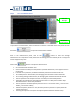
Step 4 Analyze the results The result tab displays the results of the sound transmission class to the evaluated partitions. The measurements can be saved and exported through the menu of the 10 button.
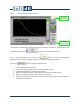
5 Main Interface Figure 1: Main interface Main controls and indicators Standard used for the STC evaluation. The standard can be changed at any time. The only difference is the frequency span used for the display and for the global value evaluation. • • ASTM E336-05, bands from 125 to 4000 Hz ISO 140-4, bands from 100 to 3150 Hz Main interface tabs: • • • Measurements tab (section 7, p.16) Result tab (section8, p.24) Comments tab (section 9, p.26) File Menu button (see the following table).
File Menu New Creates a brand new measurement session. Open Opens a previous measurement file. Save Saves the current measurement into the specified file. Save As… Saves the current measurement into a new file. Export Exports the measurement data into a text file. The file is saved as .xls extension and can be opened with Microsoft Excel or any text editor. Launches the File Manager File Manager (see section 10, p. 26) Quit: Allows to quit the module and to return to the Opus Suite Interface.
6 Setup Interface Figure 2: Setup interface Input Setup The input channel used for the measurements The available input types are AC and ICP sensors. Selection of the dynamic range. For a microphone sensitivity of 50mV/Pa. - Low Range: 25 to 119 dBA - High Range: 37-130 dBA Concerto: the input 1 and 2 have two range settings (Low or High) while inputs 3 and 4 have a single fixed range (Low). Alto-6ch and Itrack: only the low range is available.
Level Measurement Setup The unit can be used to generate a pink noise or a white noise. The output signal is balanced on output 1 and output 2. If an external generator is used, the source type can be set to external. This disables the outputs. When an internal generator is used, the volume can be adjusted from 0 to 100%. The average period of the two types of level measurement can be adjusted independently. The average type of the two types of measurement can be adjusted independently.
6.1 Sensor Calibration The input sensitivity can be calibrated using the calibration function and a sensor calibrator. Click the button on the Setup interface to launch the Calibration interface. Step 1 Adjust the calibration parameters The defaults values are: • • • Averaging time: Frequency: Calibrator Level: 5s 1 kHz 94 dB Step 2 Install the calibrator device on the microphone Step 3 Click START After the average time is elapsed, the sensitivity value will update.
7 Measurements tab Details of the selected element in the table Partition Info Table of Measurements The Measurements tab can be divided in three parts. The partition information is in upper left corner. Just under is the table of measurements. Finally, the details of the selected element are on the right side. Measurements controls The partition menu let you select the partition to measure. To add a new partition, select the last element (“new…”) of the menu ring.
If an element of the table is selected, the measurement interface will be called (see the following subsections). Click this button to delete the selected table element. The import feature allows the user to load one column of data (one of the 4 data types) from another partition of the same file. It is then possible to avoid repeating the same measurements when several partitions share data with each other.
Details of the selected element in the table Name and global level of the selected element. Description of the selected element Spectrum graph of the selected element in the table.
7.1 Level Measurement Interface Level Measurement controls The Start/Pause button starts/pauses the average measurements. The measurement will stop by itself at the end of the average period. The Stop button stops the average process The Reset button restarts the average measurement. Progress bar of the average time. The average parameters of Average type and Average Period can be modified directly on the Measurement Interface.
7.2 Reverberation Measurement Interface Figure 3: Reverberation Measurement Interface Reverberation Measurement controls The Run/Pause button starts/pauses the average measurements. The measurement will stop by itself at the end of the average period. The Stop button stops the average process. The upper progress bar is the progression of the current iteration. The bottom progress bar is the progression of the iterations relative to the requested “Nbr Averages”.
Once the measurement is acceptable, press the Accept button to return to the main interface. 7.2.1 Reverberation: Time Decay This display shows the response to a noise interruption. It also superimposes the curves used to evaluate the reverberation time values and the averaged successive responses. Figure 4: Time Decay tab of the reverberation Time Decay Graph This graph displays the time decay curves for the selected frequency band or global.
7.2.2 Reverberation: Spectrum This display shows a selected result for each frequency band and global using a bar graph. To select a frequency or the global, simply click the corresponding bar. These buttons are used to select the result to display on the spectrum graph and Global Bar. This indicator displays the selected result for the global. This array displays the computed results for the selected frequency band or global.
7.2.3 Reverberation: Data This display shows all data for all frequency bands and global in a table form.
8 Result tab Details of the selected element in the table Table of Results Figure 5: Result tab The Result tab of the main interface contains the table of result (left side) and the details (right side). The table is expendable vertically as partitions are added (in the Measurements tab). Therefore, each line of the table gives the result of one partition. Table of Results Partition index. Average level in the source room while the source is turned on.
Details of the selected element in the table Name and value of the selected element. Description of the selected element Spectrum graph of the selected partition.
9 Comments tab The Comments tab on the main panel can be used as a general note pad that will be saved along with the measurement data.
10 Explorer Dialog File / Folder Operators Directory Path Shortcuts Directory Content Explorer Window Controls and Indicators File/Folder Operators Directory Path Shortcuts • • • • • Displays the path of the active directory. Accesses to common directories.
11 File Manager The File manager is used to perform most file operations: • • • • • Navigate the directory structure Create folders Rename files and folders Move or copy files and folders from one place to another Delete a file or a folder Although not very useful on a stand-alone computer, this manager is necessary on the Concerto, on which Windows explorer is unavailable.
Directory Path Displays the path of the active directory. Shortcuts • Desktop • My Documents • Computer When the File Manager is used on a Concerto, the shortcuts are linked to: Allows easy access to common directories. When the File Manager is used on a stand-alone computer, these shortcuts are linked to: • • Move/Copy Operators File/Folder Operators Directory Content Disk info Opus Root USB Device. Copies or moves a file or folder from a source to its destination.
Appendix 1: Concerto Hardware Connections Mic Stand 4 Inputs Loudspeaker Headphone Jack Power-on button 2 Outputs DC in ¼ 20 insert Second Battery USB port Battery indicator Right click 30 Enter Arrow keys
Power on/off Power-on Turn On Turn Off Press the trigger button located at the back of the unit This key has two (2) functions: 1. To turn the unit ON. 2. Start a measurement once the SLM Module is loaded After a few seconds, the Opus Environment Interface will appear. The stand-by mode allows fast load time. Stand-by • To put the unit on stand-by, click the Turn Off button.
Power Reset If the Concerto happens to crash and it is not possible to take back the control, a power reset might be necessary. To complete the power reset, the three buttons on the front of the Concerto must be used. Here is the procedure: Step 1 Press and hold the Function, Enter and Down Arrow button for 5 seconds until the Concerto shuts down Step 2 Wait 5 seconds and press the power button Step 3 Wait 5 seconds and press the power button a second time to restart the Concerto from a power reset.
Inputs and Signal Processing Specifications (Embedded Signal Ranger MK3 DSP Board) Texas Instruments TMS320C6424 DSP Processor 4 Inputs 2 Outputs 2 x (25-120 dBA or 30-130 dBA) + 2 x (25-120 dBA) Linear Range AC, DC, ICP (4 mA) Conditioning Physical (DAP Tech 9000 Tablet PC) Intel Atom E660T 1.3 GHz Operating system Storage Data Transfer 16 GB SSD USB Display 180 mm (7 inches) WVGA (800 x 480) Dimensions 230 x 185 x 60mm (9.0 x 7.3 x 2.
Appendix 2: 1/3 Octave Filters – IEC 61260 Class 1/ANSI S1.11 1/3 Octave Filters The 1/3 octave filters are computed at low-level in real time (at 48 kHz) on the digital signal processor (DSP) of the Concerto system. The filters comply with all requirements of IEC 61260 for Class 1. Frequency Range 20 Hz to 20 kHz. Filter Shape The following curve presents the filter shape test done for the 1000 Hz 1/3 octave band. The red and green curves represent the limits associated with the IEC standard (Class 1).
Shape Test Numerical Results at 1 kHz The following table presents the numerical results of the shape test at 1 kHz: Frequency (Hz) Low limit (dB) Measurement (dB) High limit (dB) 185.5 -inf -96.0 -75.0 327.5 -inf -85.1 -62.0 531.4 -inf -61.1 -42.5 772.6 -inf -28.2 -18.0 891.3 -4.5 -3.0 -2.3 919.6 -1.1 -0.3 0.15 947.0 -0.4 0.0 0.15 974.0 -0.2 0.0 0.15 1000.0 -0.15 0.0 0.15 1026.7 -0.2 0.0 0.15 1055.8 -0.4 0.0 0.15 1087.5 -1.1 -0.3 0.15 1122.0 -4.5 -3.
1/3 Octave Filter Linearity The linearity of the 1/3-octave filter has been measured for both ranges (low and high). The experimentation is done with an adaptor (ADP092) and an electric signal. The results in dB are for an input sensitivity of 50 mV/Pa. The maximum and the minimum linear levels are measured for each 1/3 octave band along with the noise floor. Filter Linearity (Low Range) Saturation Level Frequency (Hz) (dB) 120.5 20 Minimum Linear Level (dB) 39.5 Linear Dynamic Range (dB) 81.
Minimum Linear Level (dB) 27.0 Linear Dynamic Range (dB) 93.5 Noise Floor (dB) 12500 Saturation Level (dB) 120.5 16000 120.5 27.6 92.9 19.5 20000 120.5 28.3 92.2 19.7 Minimum Linear Level (dB) 51.5 Linear Dynamic Range (dB) 81.0 Noise Floor (dB) Frequency (Hz) Filter Linearity (High Range) Saturation Level Frequency (Hz) (dB) 132.5 20 17.5 7.3 25 132.5 49.2 83.3 5.3 31.5 132.5 47.1 85.4 2.0 40 132.5 44.2 88.3 7.9 50 132.5 41.8 90.7 9.3 63 132.5 39.1 93.4 9.
Minimum Linear Level (dB) 33.5 Linear Dynamic Range (dB) 99.0 Noise Floor (dB) 10000 Saturation Level (dB) 132.5 12500 132.5 34.1 98.4 25.2 16000 132.5 35.8 96.7 27.3 20000 132.5 37.1 95.4 27.7 Frequency (Hz) 23.5 1/3 Octave Filter Summation For this test, sine waves from 20 Hz to 20 kHz are measured with the Concerto system. For each sine wave the summation of the 1/3 octave filters is computed to form the following curves. The sine waves are electrical signals at 1 VRMS.
Summation Test (High Range Case) 0.5 0.4 0.3 Amplitude dB 0.2 0.1 0 -0.1 -0.2 -0.3 -0.4 -0.